Frequently Asked Questions

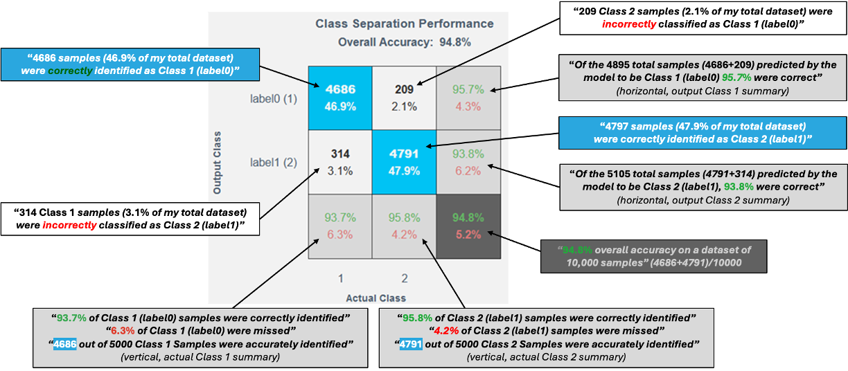
How to read a confusion matrix?

A confusion matrix is used to evaluate how well a trained classifier performs.

Matrix Layout

• Rows → Predicted class (what the model predicted)
• Columns → Actual class (ground truth from data)

Key Elements

• Diagonal cells (blue)
  Correct predictions
  • True Positive – Correctly predicted positive class
  • True Negative – Correctly predicted negative class
• Off-diagonal cells (white)
  Incorrect predictions
  • False Positives and False Negatives
  • In multi-class models, these highlight class confusions

Marginal Information

• Bottom row → Per-class accuracy (green) and error rate (red)
• Bottom-right corner → Overall model accuracy and error rate

Axis Label Mapping

• X-axis numbers map directly to Y-axis class labels
  Example: If fan-balance (1) is on the Y-axis, then 1 on the X-axis refers to the same class.

Data Representation

• Each value maps to a corresponding data segment in the histograms.

What makes a good confusion matrix?

A good confusion matrix typically shows:

• Very small values in off-diagonal (white) cells
• Strong dominance along the diagonal, indicating correct predictions

NOTE

A confusion matrix highlights not just accuracy, but where the model makes mistakes—making it a powerful tool for model improvement.

How should I interpret the complexity numbers?

Complexity numbers indicate the resource usage of a model when deployed on an MCU / MPU.

• These values are not final
• Models can often be further optimized

Example If the decision significance plot shows that most important frequency bands are below 50 Hz:

• Apply a filter to use only < 50 Hz frequencies
• Reduce feature computation
• Save multiplication operations and memory

NOTE

If a target processor was selected during project creation, the top models already fit within that processor’s available resource limits.

What is one-vs-one classification strategy?

One-vs-One is a strategy commonly used for multi-class classification.

How it works

• A binary classifier is trained for every pair of classes
• For N classes → N(N−1)/2 classifiers

Example For classes A, B, C, the model trains:

• A vs B
• A vs C
• B vs C

Prediction Phase

• All classifiers run in parallel
• Final class is chosen using a voting or aggregation mechanism

Why it’s useful

• Simplifies complex multi-class problems
• Often improves accuracy and interpretability

How does neural network model compression work?

Neural network models are often larger and more complex than necessary. Before training with real data, it is difficult to determine the exact size or architecture a model requires.

Model compression addresses this by identifying redundant or underused weights in the network and removing them. Using our proprietary mathematical approach, we detect these redundancies and restructure the network to make it simpler, smaller, and faster.

Throughout this process, we carefully balance compression with accuracy to ensure that important information is not lost.