Curate
- Version 5.6.6
- Version 6.0
Introduction
The Curate page is where most of the pre-processing work is performed. Here, all the source files will be parsed into discrete samples of consistent size. Then, all samples will be added to a sample list. This section contains two sub-tabs: Source Files and Data Sample Lists.
- Source Files: This is where you manage the raw data collected during your project.
- Data Sample Lists: Here, you create smaller, curated datasets from the available source files.
When collecting data for extended periods, the resulting files are often too large for microcontroller units with limited memory and processing power. These devices are designed to handle smaller, focused datasets, enabling them to process only critical instances where meaningful events occur.
The Curate page helps to achieve this by breaking down large data files into smaller, manageable pieces. This process ensures that the model can be trained effectively to mimic real-world scenarios, optimizing its performance for deployment in constrained environments. Breaking down the data files is important as these blocks will be the input to your ML model. For example, if your data files is 10 seconds long, you can break it down into 10 segments, 1 second long each. We can choose the length of these segments based on prior knowledge of a use-case or start with a 1 second window length and experiment from there.
Source Files
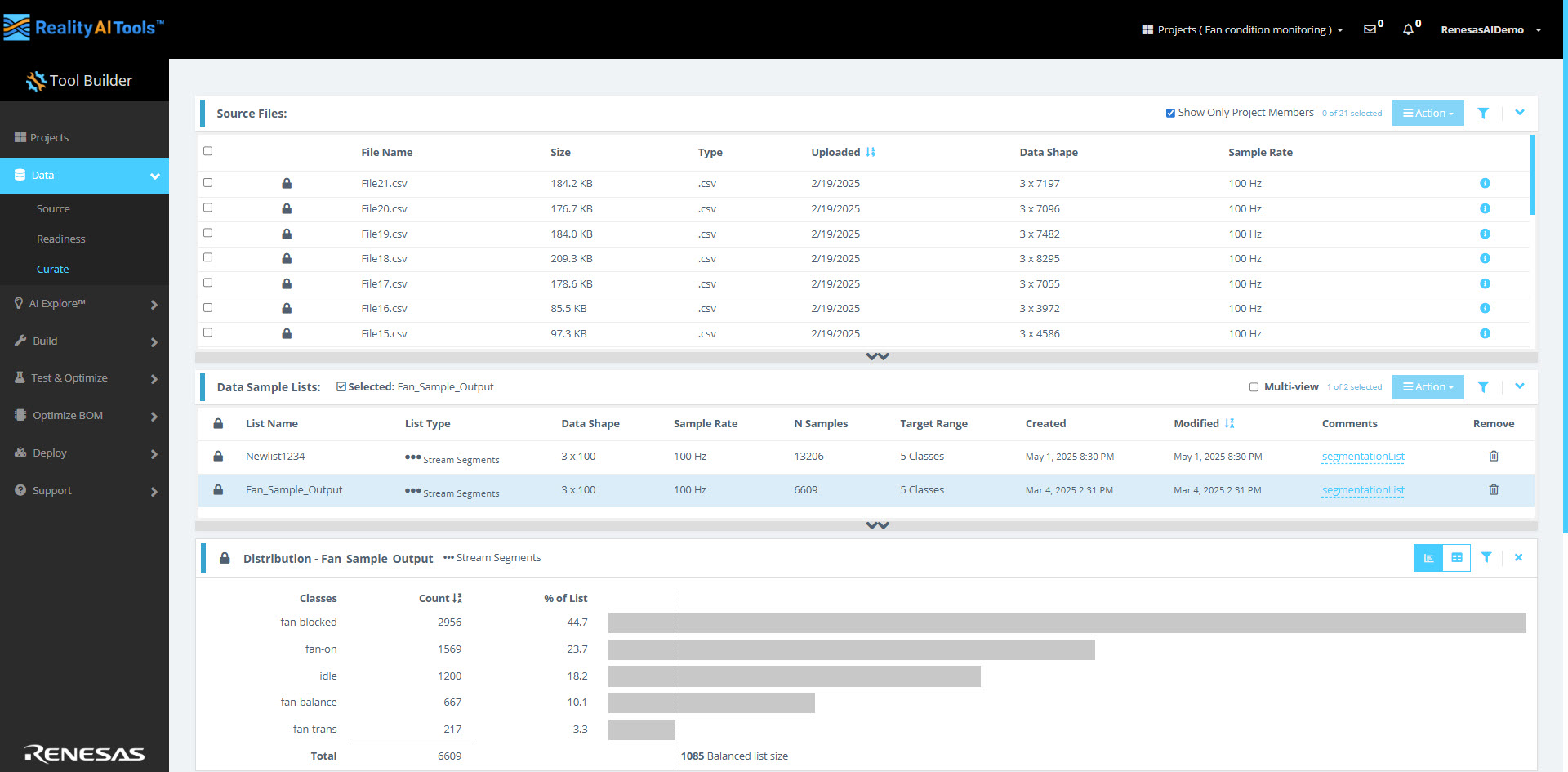
Here, you can see all the uploaded data files along with their File Name, Size, Type, Uploaded date, Data Shape and Sample Rate.
Viewing Project Members
Select the Show Only Project Members checkbox to filter the source files displayed, limiting the view to files associated with project members only.
Actions
In the Action dropdown menu, you’ll find the following options:
- Select All: Select all files listed.
- Deselect All: Clear all selected files.
- New List From Selected: Create a new list using the selected files.
- Segment List From Selected: Create a segmented list from the selected files.
- Edit Metadata Type: Modify the metadata type for the selected files.
- Format Selected: Define or update the file format for the selected files.
- Remove Selected: Remove the selected files from the project.
- Import Metadata: Upload a metadata file to add or update metadata for the source files.
- Close: Exit the action menu without making changes.
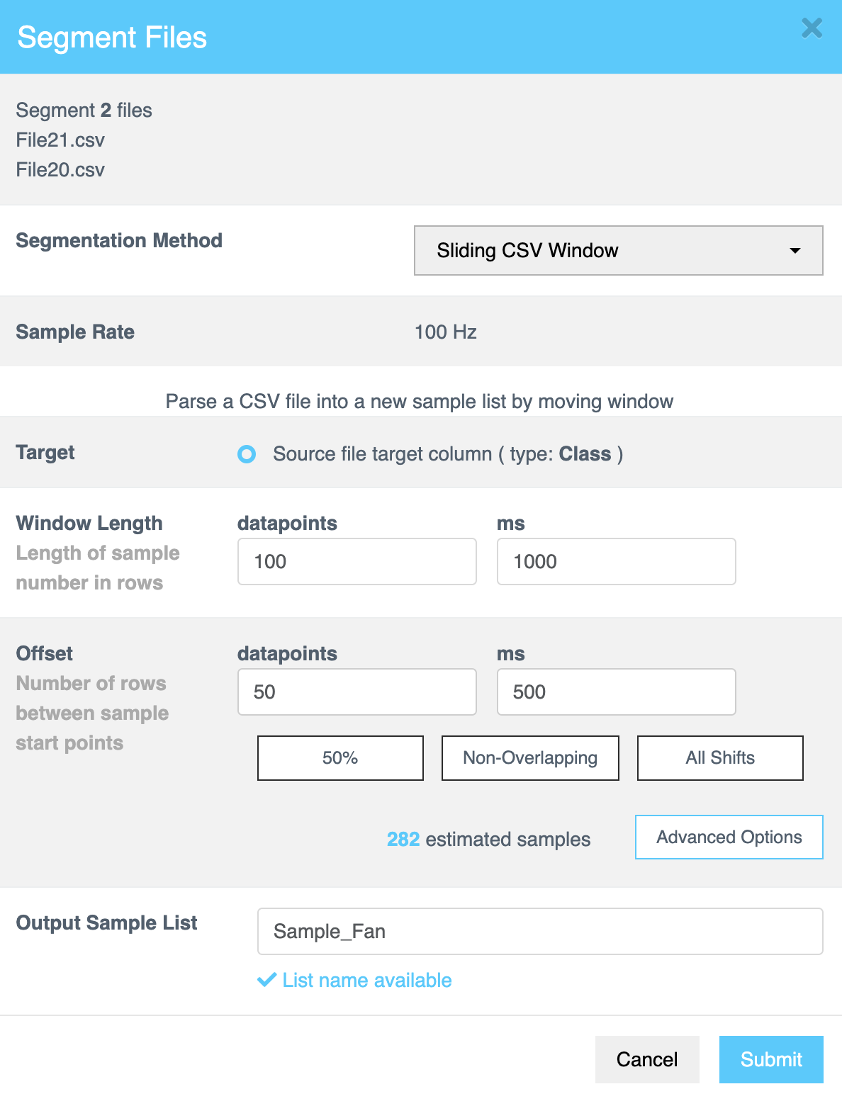
Creating a Segmented List
After labeling your files, you can create a segmented list to divide your data into smaller, manageable samples for analysis and training. Follow these steps to configure the segmentation method and options effectively.
Why segmentation?
Segmentation plays a crucial role in generating models that are optimized for deployment in resource-constrained environments, such as those using microcontrollers (MCUs). These models are designed to process live data quickly and efficiently, often within small time windows, such as 1 second, 500 milliseconds, or even shorter durations.
In real-world applications, models need to make predictions based on short, continuous streams of data rather than long, uninterrupted recordings. To replicate this scenario during the training phase, raw data is divided into smaller segments. These segments are then used to train the model, enabling it to learn and adapt to the type of data it will encounter in live, production environments.
This approach ensures the model performs effectively in real-time scenarios while operating within the constraints of limited processing power and memory.
Steps to Create a Segmented List
- Go to Actions > Segment List from Selected.
- The Segment Files window opens, displaying the selected files for segmentation.
- From the Segmentation Method dropdown menu, choose one of the following methods:
- Sliding CSV Window
- Energy Triggered
Sliding CSV Window Configuration
The Sliding CSV Window method divides CSV data [numerical, text based or time series data] into smaller, manageable samples using a step-by-step sliding window approach throughout the file, capturing data in each step until the entire file is processed. The table below summarizes the configuration options available for this method:
Option | Description |
|---|---|
Sample Rate | Displays the fixed sampling rate for parsing the CSV file into a sample list. This value is fixed during the file formatting. |
Target | Select the target column from the file metadata (type: Class). |
Window Length | The Window Length determines the size of the decision window used for segmentation. Specify the length of each sample in rows or milliseconds (ms). This value controls how much data the AI analyzes to classify each segment. Tip: Experiment with different window lengths to identify the best configuration for your dataset. |
Offset | The Offset specifies the gap between the starting points of consecutive samples within the source file. Enter the value in rows or milliseconds (ms) to define how far the parser moves before creating a new sample window. |
50% Overlap |
|
Non-Overlapping |
|
All Shifts |
|
Advanced Options
Customize the segmentation further by clicking Advanced Options.
| Option | Description |
|---|---|
| Restart Streamed Window | Restarts the window at the beginning of each class or metadata block. |
| Respect Transitions: Ensures transitions within class or metadata blocks are handled. | |
| Class: Handles transitions specifically within class blocks. | |
| Keep Short Window Samples | Determines how to handle short samples at the end of a file or class block. |
| Retain Short Samples: Includes short samples in the output. | |
| 1 per Block: Retains one short sample per block. | |
| Output Type | Select how to save the segmented samples: |
| Output to New List: Creates a new list for segmented samples. | |
| Append to Existing List: Adds parsed samples to an existing list. |
The Explorer Tier has a limitation that restricts the creation of segmented lists to fewer than 7,000 samples.
Output Sample List
After configuring the segmentation, provide a name for the segmented sample list on the Output Sample List page. This field is mandatory.
| Action | Description |
|---|---|
| Submit | Confirms the configuration and completes the process. |
After clicking on Submit, wait for a ~30 seconds and refresh the page. After refreshing the page, click on the Data Sample List tab. After clicking on the tab, you should be able to see the finished processed list.
It takes < 1min to segment/ break down this dataset. However, the duration of segmentation depends on the size of the dataset. For example: A 1 GB file may take 5-10 minutes to segment.
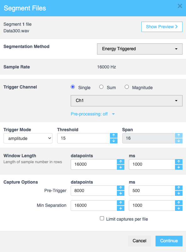
Energy triggered
When you select the energy-triggered option, you can configure the following settings as needed. This segmentation method is particularly suitable for regression datasets like audio based signals.
| Field | Description |
|---|---|
| Show/Hide Preview | Displays an overview of the data file, including the file name, selected class, trigger points, capture window, and a graphical representation of the data. This feature allows you to refresh the preview, set start and end points for the data, pan and zoom within the graphical representation, and view the full file for a comprehensive analysis. |
| Sample Rate | Sets the frequency at which data is sampled. For energy-triggered events, this is automatically set at 100 Hz to ensure accurate data capture. No manual input is required. This is fixed during file formatting. |
| Trigger Channel | Determines the source for trigger detection. Options include: |
| - Single: Select a specific channel from the dropdown menu to monitor for energy-triggered events | |
| - Sum: Allows you to combine channels mathematically (e.g., sum or difference) to define a trigger condition across multiple channels. | |
| - Magnitude: Enables monitoring of multiple channels simultaneously by calculating the combined magnitude. | |
| Pre-Processing | Configures data normalization. Select the Normalize checkbox to enable this option. This scales data to ensure uniformity and improve comparison across samples. |
| Zeroing | Adjusts the zeroing method for data processing. Options include: |
| - None: Keeps the original data without applying any zeroing adjustments. | |
| - DeMin: Adjusts the baseline of the data by subtracting the minimum value. | |
| - DeMean: Centers the data by subtracting the mean value, ensuring zero-centered data for analysis. | |
| Zero Window | Specifies the duration over which zeroing adjustments are applied. Helps manage baseline drift over the chosen window. Enter the required value or adjust using the up and down arrows. |
| Filter | Sets the filter type for data processing. Options include: |
| - None: No filter is applied to the data. | |
| - Low: Applies a low-pass filter to remove high-frequency noise, retaining lower frequencies for analysis. | |
| - Band: Applies a band-pass filter to isolate frequencies within a specified range, removing frequencies outside this band. | |
| - High: Applies a high-pass filter to remove low-frequency noise, retaining higher frequencies for analysis. | |
| Trigger Mode | Determines the mode for triggering. Options include: |
| - Amplitude: Detects triggers based on the amplitude (signal strength) of the data. | |
| - + Crossing: Triggers when the signal crosses a positive threshold. | |
| - - Crossing: Triggers when the signal crosses a negative threshold. | |
| - RMS: Uses the Root Mean Square (RMS) value for trigger detection, focusing on overall energy in the signal. | |
| - RMS Step: Triggers based on step changes in RMS values. | |
| - RMS Step Ratio: Detects triggers based on the ratio of consecutive RMS step changes. | |
| - Peak to RMS Ratio: Triggers based on the ratio of the peak signal value to its RMS value, useful for identifying transient signals. | |
| - Diff: Detects triggers based on differences between consecutive data points. | |
| - Sign: Monitors the sign (positive or negative) of the signal for trigger detection. | |
| Threshold | Specifies the minimum signal level required to trigger an event. Enter the required value or use the up and down arrows. |
| Span | Defines the duration or range for trigger detection. This field is inactive if Amplitude, Diff, or Sign is selected in Trigger Mode. |
| Window Length | Sets the number of samples in a row used for analysis. Helps control the resolution of captured data. Enter the value directly or adjust using the up and down arrows. |
| Datapoints | Specifies the number of data points to analyze within the selected window. Enter the required value or adjust using the up and down arrows. |
| ms | Defines the window length in milliseconds for temporal analysis. Enter the required value or adjust using the up and down arrows. |
| Capture Options | Configures the pre-trigger or minimum separation values for capturing data: |
| - Pre-Trigger: Determines the amount of data captured before the triggering event occurs, aiding in understanding pre-event conditions. | |
| - Min Separation: Ensures a minimum interval between successive trigger events to avoid capturing redundant data. | |
| Limit Captures Per File | Limits the number of captures stored in a single file to manage file sizes and improve data organization. Select the checkbox to activate this option. |
Click Continue to fill in more details as follows:
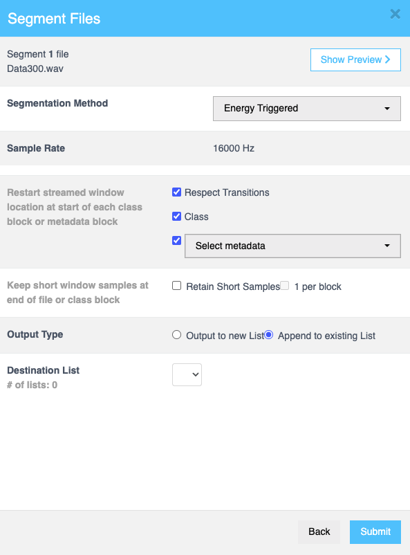
| Field | Description |
|---|---|
| Restart streamed window location at start of each class block or metadata block | When you select the Respect Transitions checkbox, the Class and Metadata checkboxes become editable. If you select Metadata, a dropdown appears, allowing you to specify the required metadata.. |
| Keep short window samples at end of file or class block | Select the Retain Short Samples checkbox to keep short samples at the end of a file or class block. You can also enable the 1 per block checkbox to retain one short sample per block. |
| Output type | Choose between Output to new List or Append to existing List using radio buttons to determine whether to create a new list or add results to an existing list. |
| Output Sample List | This field is available if you select Output to new List. Enter the name of the output list where the processed samples will be saved. |
| Destination List | This field is available if you select Append to existing List. Select the required lists from the dropdown menu. |
Click Submit to confirm.
Filtering Source Files
- Click the Filter icon to open the Filter Source Files page.
- Use the available filters to narrow your search:
- Name: Search files by name.
- Data Type: Filter based on the data type.
- Date: Filter by file creation or modification date.
- Data Shape: Narrow down files based on data shape.
- Sample Rate: Filter by the sample rate.
- Unformatted: Find files that are yet to be formatted.
- Assigned Targets: Filter files with assigned targets.
- Unassigned Targets: Locate files with no targets assigned.
- After filling in the required fields, click Apply to filter the source files.
Defining the Target Class
To define the target class for your data, you have two options:
- Using an Additional Column in the Source File: While uploading a source file, include an extra column that specifies the label for each data point.
- Using a Metadata File: Prepare a CSV file named metadata with the following two columns:
-
- File Name: A list of all the file names you have uploaded.
- Label Type: The corresponding label for each file.
- File Name: A list of all the file names you have uploaded.
-
For example, if you have 10 files for "apples" and 5 files for "oranges," assign the labels accordingly in the metadata file.
Importing Metadata
- On the Curate page, in the Source Files tab, use the Action > Import Metadata option to upload the metadata file.
- A dialog box will appear, allowing you to drag and drop the prepared CSV file.
- Select Target Value from the second row dropdown. Keep the first row dropdown as File Names. This will label the files according to the assigned metadata.
- Once uploaded, descriptive metadata will be added to the source files.
Viewing the Target Class
After importing metadata, expand the arrows next to the Sample Rate row. The Amps column will display the target class selection for all files.
This method is particularly beneficial when dealing with large batches of files, as adding an additional column to each source file manually can be tedious.
Data Sample Lists
This section explains how to work with Output Sample Lists, which are generated after performing the Segment List from Selected action. These lists are displayed in a tabular format with the following details:
| Field | Description |
|---|---|
| List Name | The name of the sample list. |
| List Type | Specifies the type of the list, such as classification or regression. |
| Data Shape | The shape or dimensions of the data in the list. |
| Sample Rate | The rate at which samples were collected. |
| N Samples | The number of samples in the list. |
| Target Range | The range of target values in the list. |
| Created | The date and time the list was created. |
| Modified | The date and time the list was last updated. |
| Comments | Allows you to add comments or notes regarding the data sample list. |
| Remove | Enables you to delete a specific sample list from the table. |
Multi-view Option
In the toolbar, select the Multi-view checkbox to compare and analyze lists more effectively, you can display them in multiple views.
Actions
Use the Actions dropdown menu to manage sample lists. The following actions are available:
| Action | Description |
|---|---|
| Deselect All | Clears all selected items. |
| Random Subset to New | Creates a new list from a random subset of the selected items. |
| Edit Sensor Groups | Adjusts sensor groupings for the selected lists. |
| Convert to Regression List/ Convert to Classification List | Converts the selected classification lists into regression list or vice versa. |
| Remap Classes | Reassigns class labels in the selected lists. |
| Export to CSV | Saves the selected lists as a CSV file. |
| Import From CSV | Uploads a CSV file to add or update data sample lists. |
| Close | Closes the action menu without making changes. |
| Remove Selected | Deletes the selected data sample lists. |
Filtering Lists
You can filter sample lists to find specific items.
- Click the Filter icon to open the Filter Lists page.
- Use the provided options to filter the lists based on:
- Name: Search lists by name.
- List Type: Filter lists by their type.
- Date Created: Narrow down lists based on the date they were created.
- Data Shape: Filter lists by data shape.
- Sample Rate: Search for lists based on their sample rate.
- Enter the required information in the filter fields and click Apply to refine the displayed lists.
Distribution
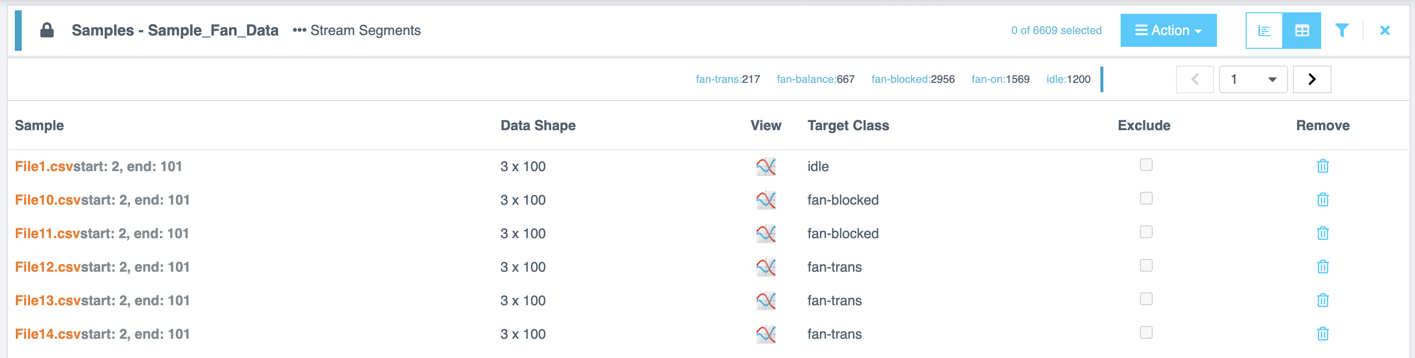
The sample lists created from segmenting the source files can be used for AI Exploration, Training or Testing. Each row contains a specific labeled sample or observation of a set length, taken from the source file stream.
Click on the newly created segmented list to view its contents. This list displays the blocks or windows of segmented data. A histogram of the data should also appear for visualization.
If the histogram does not appear immediately after segmentation, try refreshing the page.
You can analyze the distribution of a selected list in List View or Table View.
View Options
| View | Description |
|---|---|
| List View | Displays distribution details by Classes, Count, and % of List. |
| Table View | Provides detailed information for each sample, including Sample File, Data Shape, View, Target Class dropdown (to find or create a class) and Exclude and Remove options |
Perform Actions in Table View
- Select the Action button in the toolbar.
- Choose from the following options:
| Action | Description |
|---|---|
| Transfer | Transfers selected items to a different list. |
| Transfer to New List | Creates a new list from the selected items. |
| Select All | Selects all items. |
| Select All on Page | Selects all items displayed on the current page. |
| Select Random Subset | Selects a random subset of items. |
| Deselect All | Clears all selections. |
| Set Target for Selected | Assigns a target class to the selected items. |
| Exclude Selected | Excludes the selected items from the list. |
| Include Selected | Includes previously excluded items. |
| Export to CSV | Saves the selected items to a CSV file. |
| Import CSV | Imports items from a CSV file. |
| Close | Closes the action menu without making changes. |
| Remove Selected | Deletes the selected items. |
Introduction
The Curate page is where most preprocessing work is performed before AI Exploration, Training, or Testing. On this page, source files are parsed into discrete samples of consistent size, and these samples are grouped into sample lists.
The Curate page contains three main tabs:
- Project Files - View uploaded files, manage metadata, and prepare files for data sets.
- Data Sets - Combine files into data sets, configure segmentation parameters, and manage sensor groups.
- Sample Lists - Generate and manage curated subsets of samples for model training and evaluation.
When data is collected over long periods, files can become too large to work with efficiently on microcontroller units (MCUs) with limited memory and processing power. These devices are optimized for smaller, focused data sets that capture only the most meaningful events.
The Curate page addresses this challenge by breaking large data files into smaller, manageable segments. These segments simulate the real-world operating conditions of a model deployed on an MCU, where predictions are made continuously on small sliding windows of live data.
For example, a 10-second data file can be divided into 10 segments of 1 second each. The choice of segment length depends on the use case. You can use domain knowledge (for example, a vibration pattern lasting 200 ms) or start with a 1-second default and experiment with shorter or longer windows to optimize model accuracy.
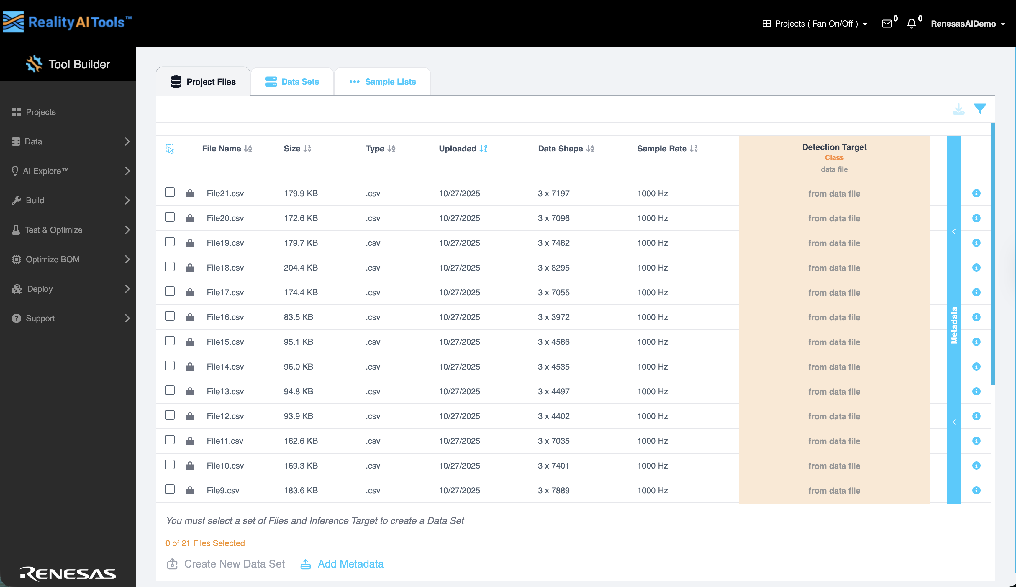
Project Files
The Project Files tab displays all uploaded data files and their associated details:
- File Name - The name of the uploaded file.
- Size - Size of the uploaded file.
- Type - Type of the uploaded file (for example, .csv).
- Uploaded - The date the file was added.
- Data Shape - The dimensional structure of the file.
- Sample Rate - The rate at which samples were collected.
- Inference Target - The label or value to be predicted.
- Metadata - Any additional descriptive information linked to the file.
Adding Metadata to Project Files
Metadata provides additional descriptive fields that can be used for filtering, labeling, or splitting data during training.
- In the Project Files tab, expand the Metadata section to view existing metadata.
- Select Add Metadata. The Add Metadata dialog opens.
- Upload a .csv file by dragging and dropping it into the dialog. This file must contain the metadata values you want to associate with your files.
Once imported, the metadata is linked to the project files and appears in the Metadata section.
Configure Import Settings
In the Add Metadata window, configure the import options to match your file format:
- Select the Label Row checkbox if your CSV includes a header row. When selected, the header row is excluded from the imported data.
- From the Delimiter dropdown, choose the column separator used in your file. Supported delimiters include Comma (,), Semicolon (;), Space ( ), and Tab (\t).
- Select the European Decimals checkbox if your file uses commas as decimal points (for example, 1.234.567,89 instead of 1,234,567.89).
- Select Confirm to finalize the import and display the metadata in the Project Files tab.
Selecting Metadata Type
Assigning correct metadata types ensures accurate data processing and model training. After uploading the metadata file:
- Select the metadata column to configure.
- Open the Select Metadata Type dropdown.
- Choose one of the following types, depending on the column content:
- Target Class - A categorical outcome label.
- Target Value - A numeric target used for regression.
- Categorical Metadata - Descriptive categorical fields (for example, machine ID).
- Numerical Metadata - Continuous numeric values.
- Sequential #s / Time Code - Ordered data such as frame or timestamp values.
- Date and Time, Date Only, or Time Only - Time-based fields.
- Ignore - Exclude a column from processing.
Once metadata types are assigned, they appear in the Project Files tab.
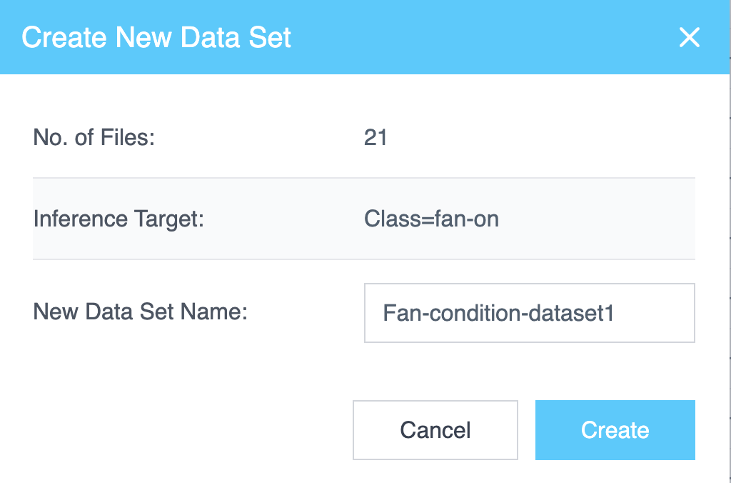
Creating a New Data Set
To create a data set:
- In the Project Files tab, select the checkbox next to each file you want to include. Multiple files can be selected.
- Select Create New Data Set.
The Create New Data Set dialog displays the following:
- Number of Files Selected
- Inference Target
- A field to enter a New Data Set Name
Enter a name and select Create to generate the data set.
If a data set already exists, the button changes to Add to Data Set. Selecting it opens a list of existing data sets, with an option to Create New Data Set. You can add selected files to an existing data set or create a new one.
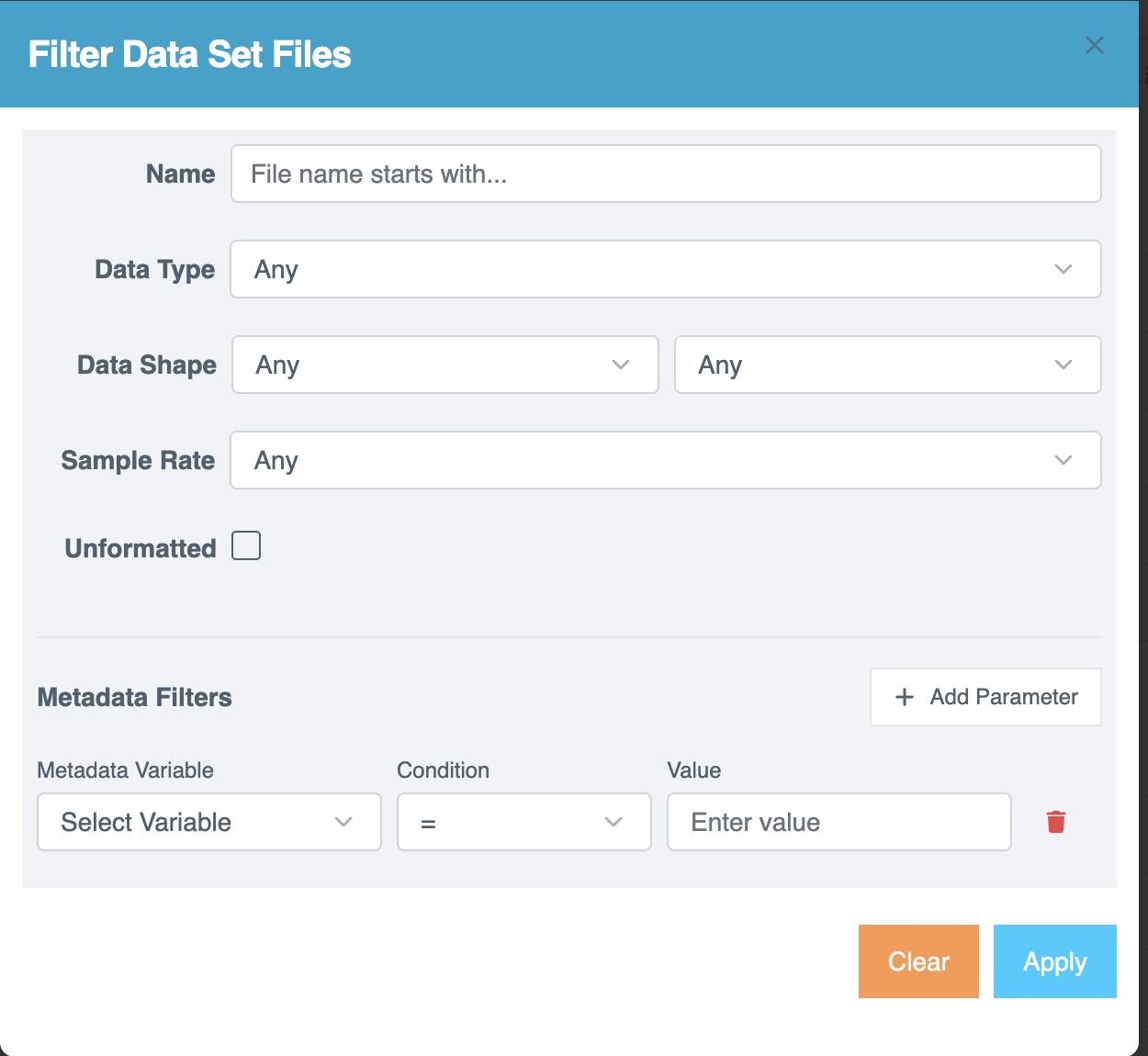
Filtering Project Files
Use filters to quickly locate files:
- Select the Filter icon to open the Filter Data Set Files page.
- Apply filters as needed:
- Name - Search by file name.
- Data Type - Filter by data type.
- Data Shape - Narrow results by data shape.
- Sample Rate - Filter by sampling rate.
- Unformatted - Identify files not yet formatted.
- Use the Metadata Filters section for advanced filtering:
- Metadata Variable - Select a variable.
- Condition - Choose an operator
(=, ≠, >, <, ≥, ≤, Contains, Starts with, Ends with, Regex). - Value - Enter the comparison value.
- Select + Add Parameter to include multiple conditions.
- Select the Trash icon to remove a condition.
- Select Apply to filter the results.
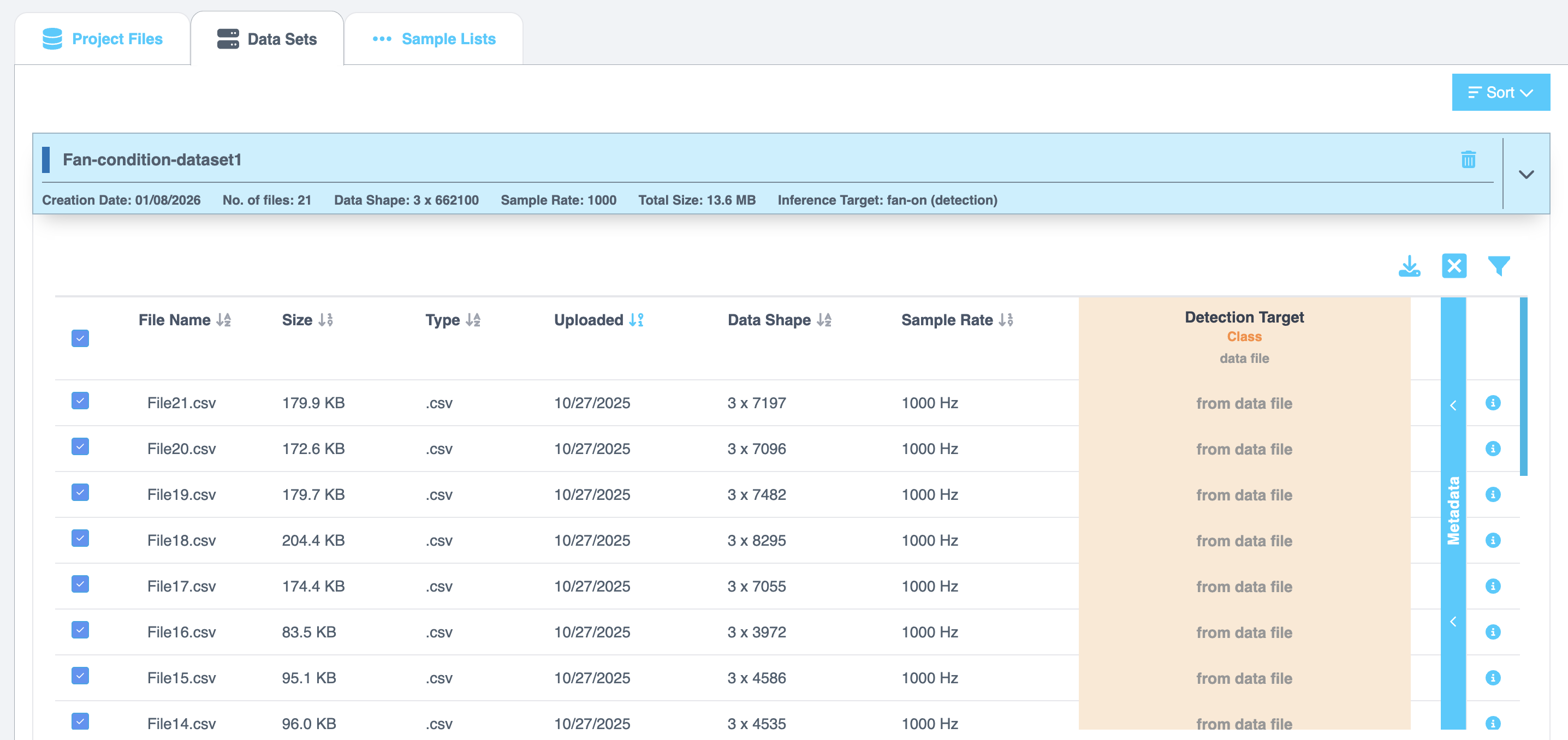
Data Sets
The Data Sets tab displays all created data sets with the following details:
- Name
- Creation Date
- Number of Files
- Data Shape
- Sample Rate
- Total Size
- Inference Target
Selecting a data set shows detailed file information, including file name, size, type, uploaded date, data shape, sample rate, inference target, and selected metadata.
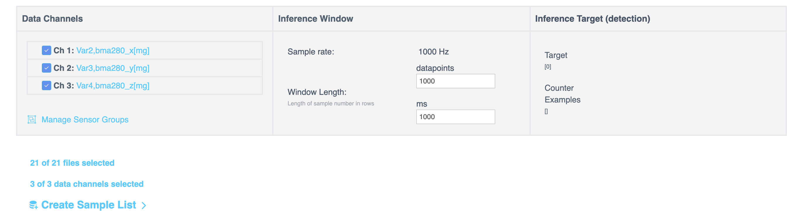
Additional Configuration Options
- Data Channels - Lists all channels in the data set. By default, all channels are selected. Use checkboxes to include or exclude channels.
- Select Manage Sensor Groups to open the Sensor Groups dialog, where you can:
- Add, rename, or delete sensor groups.
- Assign data channels to groups.
- Save changes to apply.
- Select Manage Sensor Groups to open the Sensor Groups dialog, where you can:
- Inference Window - Displays:
- Sample Rate (Hz)
- Window Length (shown in both data points and milliseconds). You can edit these values to configure segmentation.
- Inference Target - Shows the distribution of the inference target variable. The histogram is divided into bins, and you can adjust the number of bins using up/down arrows. Counts and ranges update dynamically.
At the bottom of the tab, a summary is displayed:
- Total number of files selected
- Total number of channels selected
To continue, select Create Sample List. Choose from the following:
- Single List
- Random Split
- Split by Metadata
Creating a Segmented List
Segmentation is the process of dividing raw data into smaller, uniform samples. This step is critical for training models that can operate in real time on constrained devices.
Why segmentation?
Segmentation plays a crucial role in generating models that are optimized for deployment in resource-constrained environments, such as those using microcontrollers (MCUs). These models are designed to process live data quickly and efficiently, often within small time windows, such as 1 second, 500 milliseconds, or even shorter durations.
In real-world applications, models need to make predictions based on short, continuous streams of data rather than long, uninterrupted recordings. To replicate this scenario during the training phase, raw data is divided into smaller segments. These segments are then used to train the model, enabling it to learn and adapt to the type of data it will encounter in live, production environments.
This approach ensures the model performs effectively in real-time scenarios while operating within the constraints of limited processing power and memory.
Creating a Single List
Select Single List to create one segmented list. The Segment Files to Sample List dialog opens. Configure the segmentation method, window length, and other options, then generate the list.
Creating a Random Split
Select Random Split to partition data into multiple folds for training and testing. The dialog includes
- Folds: Enter the number of folds to create. A fold is one of the partitions created when the dataset is split into multiple subsets. These folds are then used to assign data for training and testing, ensuring the model is evaluated on different portions of the dataset.
- Train: Enter the percentage of data to use for training.
- Test: Enter the percentage of data to use for testing.
Click Continue to confirm your settings. Further, the Segment files to sample list dialog opens.
Creating a Split by Metadata
Select Split by Metadata to divide data based on metadata fields such as Source File, Target Value, or user-defined metadata. The selected metadata field displays its distribution. After making your selection, the dialog displays the metadata field, its values, and the number of sample lists that will be created.
Click Continue to confirm your settings. Further, the Segment files to sample list dialog opens.
Segment Files to Sample List
This dialog configures how files are segmented into sample lists.
| Option | Description |
|---|---|
| File names | The number and names of the files to be segmented |
| Data Channels | The number and list of data channels selected in the previous section. |
The dialog updates dynamically based on the selected Segmentation Method. You can choose Sliding CSV Window or Energy Triggered.
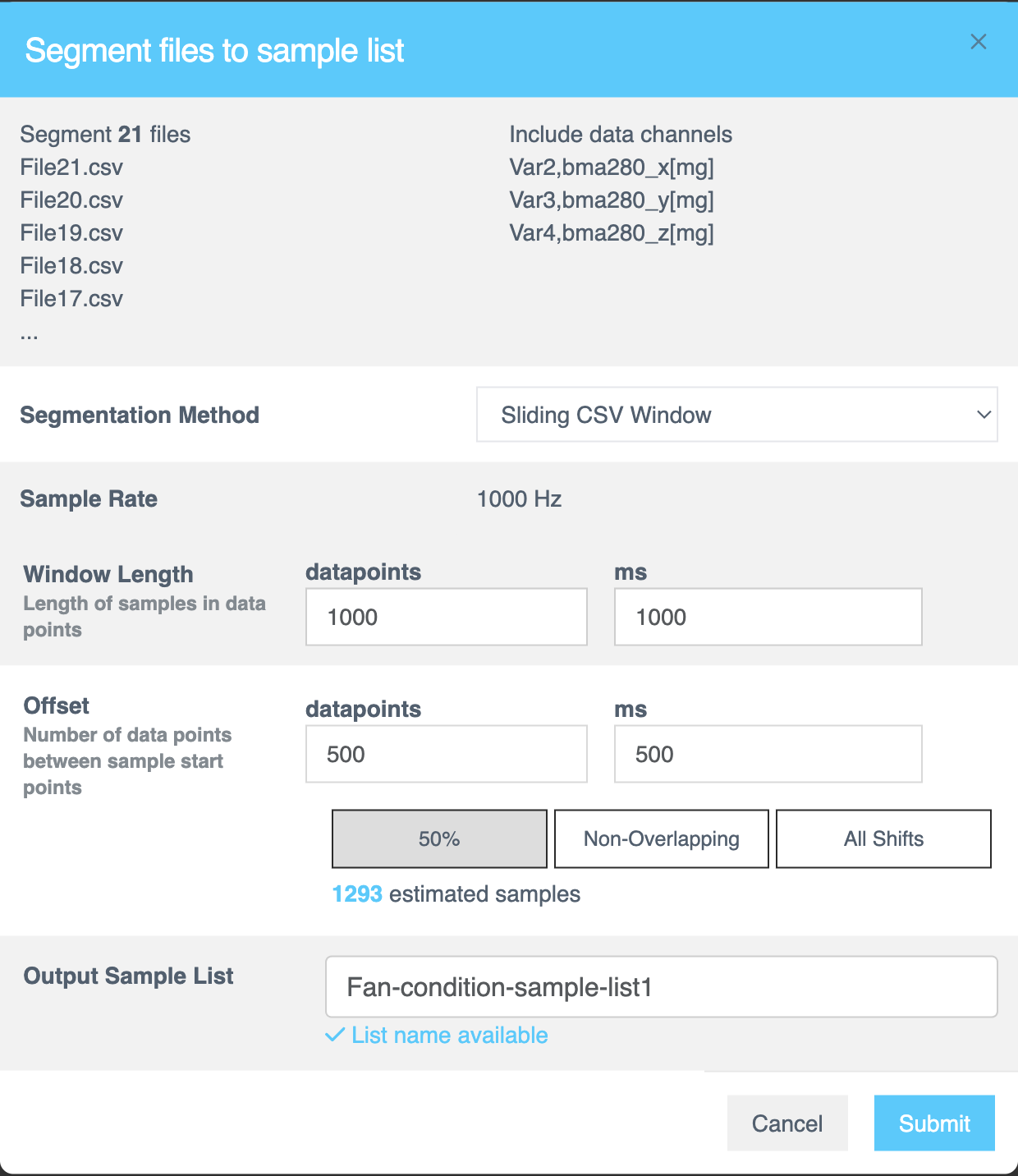
If you select Sliding CSV Window,
| Segmentation method | The Sliding CSV Window method divides CSV data [numerical, text based or time series data] into smaller, manageable samples using a step-by-step sliding window approach throughout the file, capturing data in each step until the entire file is processed. |
|---|---|
| Sample Rate | Displays the fixed sampling rate for parsing the CSV file into a sample list. This value is fixed during the file formatting. |
| Window Length | The Window Length determines the size of the decision window used for segmentation. Specify the length of each sample in rows or milliseconds (ms). This value controls how much data the AI analyzes to classify each segment. Experiment with different window lengths to identify the best configuration for your dataset. |
| Offset | The Offset specifies the gap between the starting points of consecutive samples within the source file. Enter the value in datapoints or milliseconds (ms) to define how far the parser moves before creating a new sample window. You can view the estimated samples based on the selection you make. |
| 50% Overlap | Creates samples with a 50% overlap between consecutive windows. Ensures half of the data is shared across adjacent samples. Balances the need for starting-point variation with reduced redundancy. |
| Non-Overlapping | Creates distinct samples with no shared data between consecutive windows. Suitable for datasets with a large volume of data or longer offsets. Often used during initial exploration and training. |
| All Shifts | Shifts the window one row at a time to create the maximum number of samples. Ideal for testing a finalized classifier to simulate performance on arbitrarily sampled data streams. |
| Output Sample List | After configuring the segmentation, provide a name for the segmented sample list. This field is mandatory. |
If you select Energy Triggered,
| Segmentation method | The Energy Triggered method segments data based on detected energy events within signals, capturing samples only when a trigger condition is met. This approach is particularly suited for regression datasets like audio signals, ensuring precise event-driven data analysis. |
|---|---|
| Sample Rate | Sets the frequency at which data is sampled. For energy-triggered events, this is automatically set at 100 Hz to ensure accurate data capture. No manual input is required. This is fixed during file formatting. |
| Window Length | Sets the number of samples in a row used for analysis. Helps control the resolution of captured data. Enter the value directly or adjust using the up and down arrows. |
| Trigger Channel | Determines the source for trigger detection. Options include: |
| Single: Select a specific channel from the dropdown menu to monitor for energy-triggered events | |
| Sum: Allows you to combine channels mathematically (e.g., sum or difference) to define a trigger condition across multiple channels. | |
| Magnitude: Enables monitoring of multiple channels simultaneously by calculating the combined magnitude. | |
| Pre-Processing | Configures data normalization. Select the Normalize checkbox to enable this option. This scales data to ensure uniformity and improve comparison across samples. |
| Zeroing | Adjusts the zeroing method for data processing. Options include: |
| None: Keeps the original data without applying any zeroing adjustments. | |
| DeMin: Adjusts the baseline of the data by subtracting the minimum value. | |
| DeMean: Centers the data by subtracting the mean value, ensuring zero-centered data for analysis. | |
| Zero Window | Specifies the duration over which zeroing adjustments are applied. Helps manage baseline drift over the chosen window. Enter the required value or adjust using the up and down arrows. |
| Filter | Sets the filter type for data processing. Options include: |
| None: No filter is applied to the data. | |
| Low: Applies a low-pass filter to remove high-frequency noise, retaining lower frequencies for analysis. | |
| Band: Applies a band-pass filter to isolate frequencies within a specified range, removing frequencies outside this band. | |
| High: Applies a high-pass filter to remove low-frequency noise, retaining higher frequencies for analysis. | |
| Trigger Mode | Determines the mode for triggering. Options include: |
| Amplitude: Detects triggers based on the amplitude (signal strength) of the data. | |
| + Crossing: Triggers when the signal crosses a positive threshold. | |
| - Crossing: Triggers when the signal crosses a negative threshold. | |
| RMS: Uses the Root Mean Square (RMS) value for trigger detection, focusing on overall energy in the signal. | |
| RMS Step: Triggers based on step changes in RMS values. | |
| RMS Step Ratio: Detects triggers based on the ratio of consecutive RMS step changes. | |
| Peak to RMS Ratio: Triggers based on the ratio of the peak signal value to its RMS value, useful for identifying transient signals. | |
| Diff: Detects triggers based on differences between consecutive data points. | |
| Sign: Monitors the sign (positive or negative) of the signal for trigger detection. | |
| Threshold | Specifies the minimum signal level required to trigger an event. Enter the required value or use the up and down arrows. |
| Span | Defines the duration or range for trigger detection. This field is inactive if Amplitude, Diff, or Sign is selected in Trigger Mode. |
| Capture Options | Configures the pre-trigger or minimum separation values for capturing data: |
| Pre-Trigger: Determines the amount of data captured before the triggering event occurs, aiding in understanding pre-event conditions. | |
| Min Separation: Ensures a minimum interval between successive trigger events to avoid capturing redundant data. | |
| Limit Captures Per File | Limits the number of captures stored in a single file to manage file sizes and improve data organization. Select the checkbox to activate this option. |
| Output Sample List | After configuring the segmentation, provide a name for the segmented sample list. This field is mandatory. |
On the right panel, you can preview the selected file. The orange line represents trigger points, and the blue line represents the capture window. You can view multiple channels along with an overview that supports zooming. To zoom in, select and drag a section in the overview; the zoomed view appears in the channel display above.
Select Refresh Preview to update the view.
The Explorer Tier has a limitation that restricts the creation of segmented lists to fewer than 7,000 samples.
| Action | Description |
|---|---|
| Submit | Confirms the configuration and completes the process. |
After clicking on Submit, wait for a ~30 seconds and refresh the page. After refreshing the page, click on the Data Sample List tab. After clicking on the tab, you should be able to see the finished processed list.
It takes < 1min to segment/ break down this dataset. However, the duration of segmentation depends on the size of the dataset. For example: A 1 GB file may take 5-10 minutes to segment.
Sorting Data Sets
You can sort datasets using the Sort option in the top-right corner. Available options include:
- Creation Date (Old - New)
- Creation Date (New - Old)
- Inference Target
- Sample Rate
- Data Shape
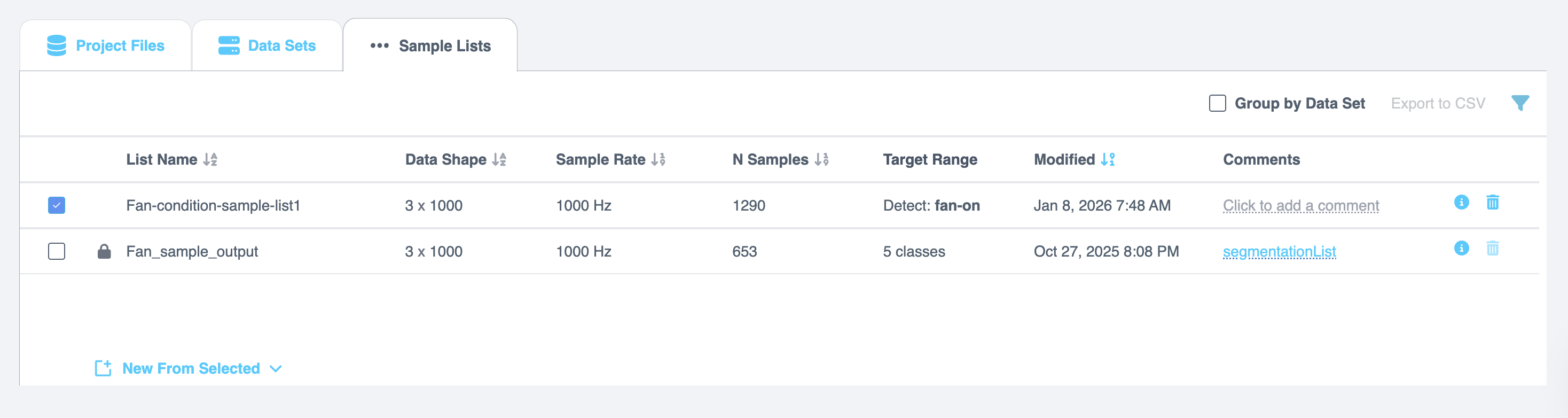
Sample Lists
This section explains how to work with Sample Lists, which are generated after performing the Segment List from Selected action. These lists are displayed in a tabular format with the following details:
| Field | Description |
|---|---|
| List Name | The name of the sample list. |
| Data Shape | The shape or dimensions of the data in the list. |
| Sample Rate | The rate at which samples were collected. |
| N Samples | The number of samples in the list. |
| Target Range | The range of target values in the list. |
| Modified | The date and time the list was last updated. |
| Comments | Allows you to add comments or notes regarding the data sample list. |
| Info | Select the Info icon to view details such as name, inference window, sample rate, shape, offset, data channels, and file names. |
| Remove | Select the Trash can icon to delete the sample list. |
Managing Sample Lists
Group by Data Set
Select the Group by Data Set checkbox to organize the sample lists by data set groups.
Create a New List from Selected Rows
- Select one or more rows from the sample list.
- Open the New from selected drop-down menu.
- Choose one of the following options:
- Copy Sample List - Creates a copy of the selected list.
- Random Subset - Creates a new list containing a random subset of the selected samples.
- Concatenate - Combines the selected lists into a single list.
Copy Sample List
When you select Copy Sample List, the Copy to New List window opens.
- Enter a new name in the List Name field.
- Select Create to generate the copied list.
Random Subset
When you select Random Subset, the Random Subset to New List window opens.
- Enter a new name in the List Name field.
- Enter a value for # of Samples per Class. This value must be less than the total number of samples.
- Select Create to generate the new list.
Concatenate Lists
When you select Concatenate, the Concatenate Lists window opens and displays the names of the selected data sets.
- Enter a new name in the List Name field.
- Select Create to generate the concatenated list.
Download as CSV
Select the Download option in the top-right corner of the table to download the sample list as a .csv file.
Filtering Lists
You can filter sample lists to find specific items.
- Click the Filter icon to open the Filter Lists page.
- Use the provided options to filter the lists based on:
- Name: Search lists by name.
- Date Created: Select a date range or choose from preset options such as Today, Yesterday, Last 7 Days, Last 30 Days, Current Month, Previous Month, or Last Year. Select Apply to confirm.
- Data Shape: Filter lists by data shape.
- Sample Rate: Search for lists based on their sample rate.
- Enter the required information in the filter fields and click Apply to refine the displayed lists.
Distribution
The Distribution section provides a visual and tabular representation of segmented sample lists created from the source files. These lists can be used for AI Exploration, Training, or Testing.
Each row in the sample list represents a labeled observation of fixed length, taken from the source file stream.
Viewing the Distribution
- Click the newly created segmented list to open its contents.
- The list displays segmented data blocks (also called windows).
- A histogram of the data appears to help visualize distribution.
- Use the # of Bins field to adjust the granularity of the histogram.
- Increasing or decreasing the number of bins updates the histogram dynamically.
- The Classes and Count fields adjust automatically to reflect the change.
- To view a graphical representation of the sample list, click the graph icon in the top-right corner of the Distribution section.
- The graph appears in a pop-up window.
- Select a sample list from the table on the left. The corresponding graph is displayed on the right.
Graph Details
The graph pop-up provides detailed information, including:
- Number of samples
- Classes and sample counts
- File name
- Start and end times (or is it values?)
- Target class
- Metadata fields
- Start and end values for each metadata field
When you select a row in the table, column-wise graphs appear along with an overview section.
Multi-Channel and Zoom Features
- You can view multiple data channels simultaneously.
- The overview panel supports interactive zooming.
- To zoom in, click and drag across the desired section in the overview.
- The zoomed-in region is displayed in the channel graph above.
- To reset, click Reset Zoom.
If the histogram does not appear immediately after segmentation, try refreshing the page.