Continuous value prediction
Introduction
This tutorial provides a step-by-step guide to using Renesas's Reality AI Tools portal for building AI models in non-visual sensing applications. We will work with a continuous value dataset collected from a vibration sensor to predict exact numerical values rather than categorical classifications.
Objectives
By the end of this tutorial, you will:
- Gain hands-on experience with the Reality AI Tools – Values module.
- Learn how to analyze and develop machine learning models for non-visual sensing applications.
Requirements
Hardware & Software
- A PC or MacBook with Chrome or Firefox installed.
Dataset
- 250 CSV files containing continuous value data. Click here to download: CV Prediction Dataset
- 1 metadata.csv file. Click here to download: CV Prediction Metadata
Estimated Time
60 minutes
Step 1: Creating a Project and Uploading the Dataset
Step 1.1: Accessing Reality AI Tools
- Open your web browser and go to: portal.reality.ai.
- Enter your login credentials (provided via email) and click Login.
Step 1.2: Creating a New Project
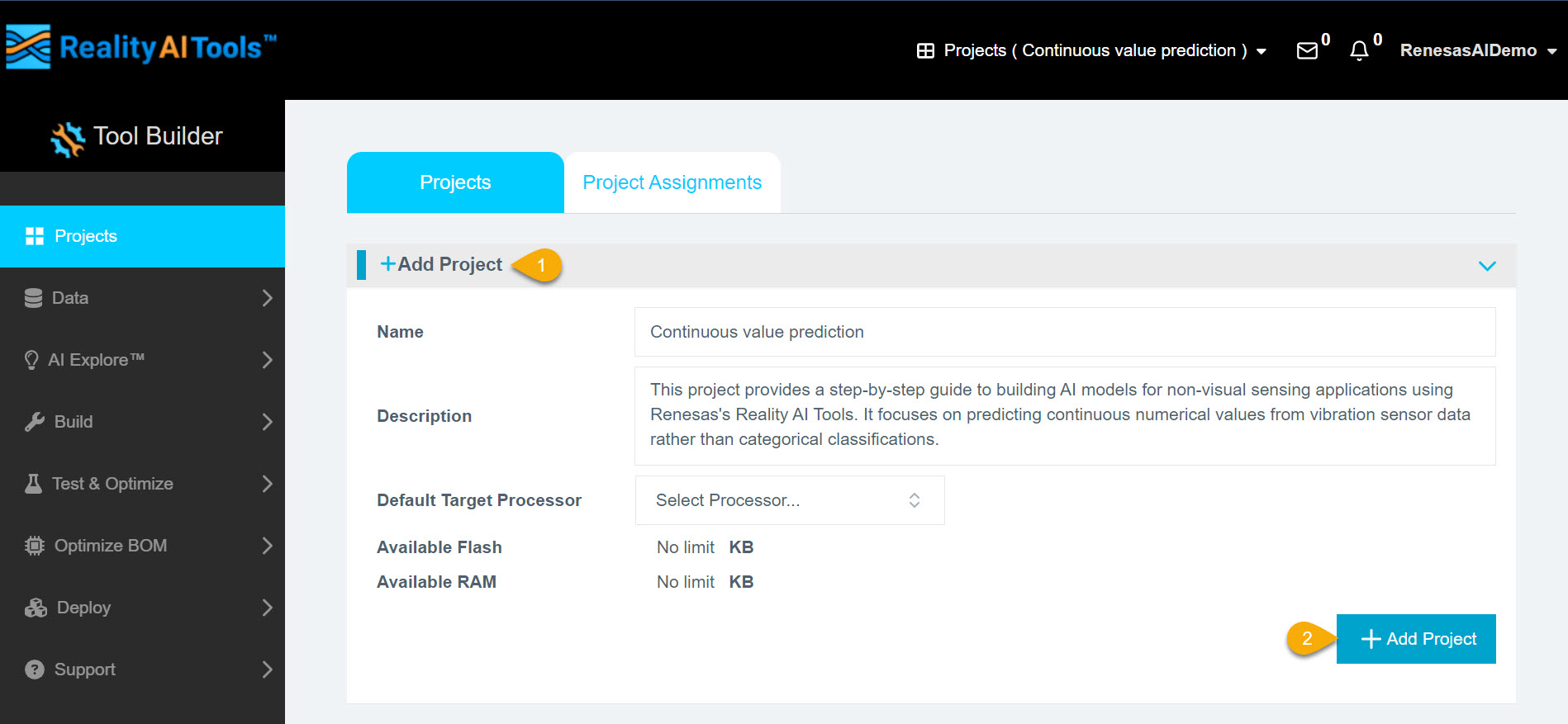
- After logging in, the Reality AI Tools portal will open with no projects listed.
- Click Add Project and enter the following details:
- Project Name (required)
- Description (optional)
- Click Add Project to proceed.
Step 1.3: Selecting the Project
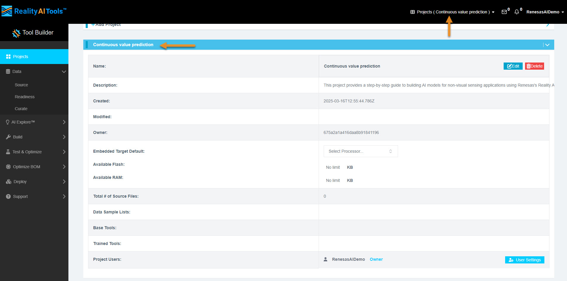
- Once the project is created, click its name to open it.
- This will allow you to manage datasets and perform various analyses.
Step 1.4: Uploading the Dataset
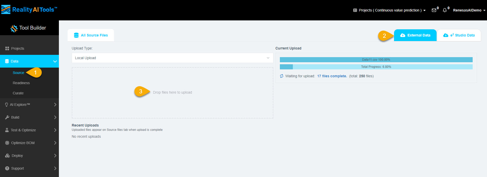
- In the left menu, click Data > Source.
- Navigate to the External Data tab.
- Click Drop file here to upload and select the dataset files.
Step 1.5: Selecting Files for Upload
- Navigate to the downloaded dataset folder.
- Select all 250 data files.
- Click Open to upload them to the portal.
- The file upload progress will be displayed on the page. Wait for all files to be fully uploaded.
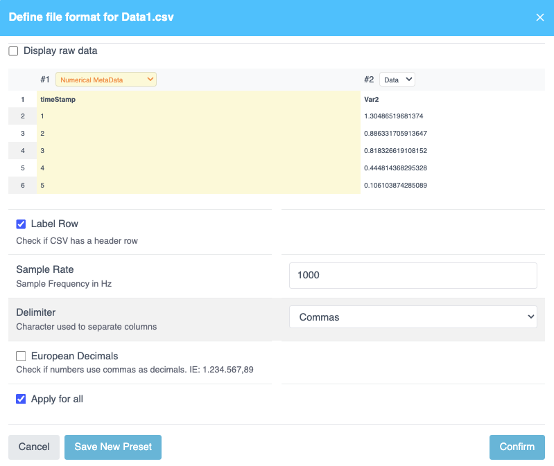
Step 1.6: Formatting the Dataset
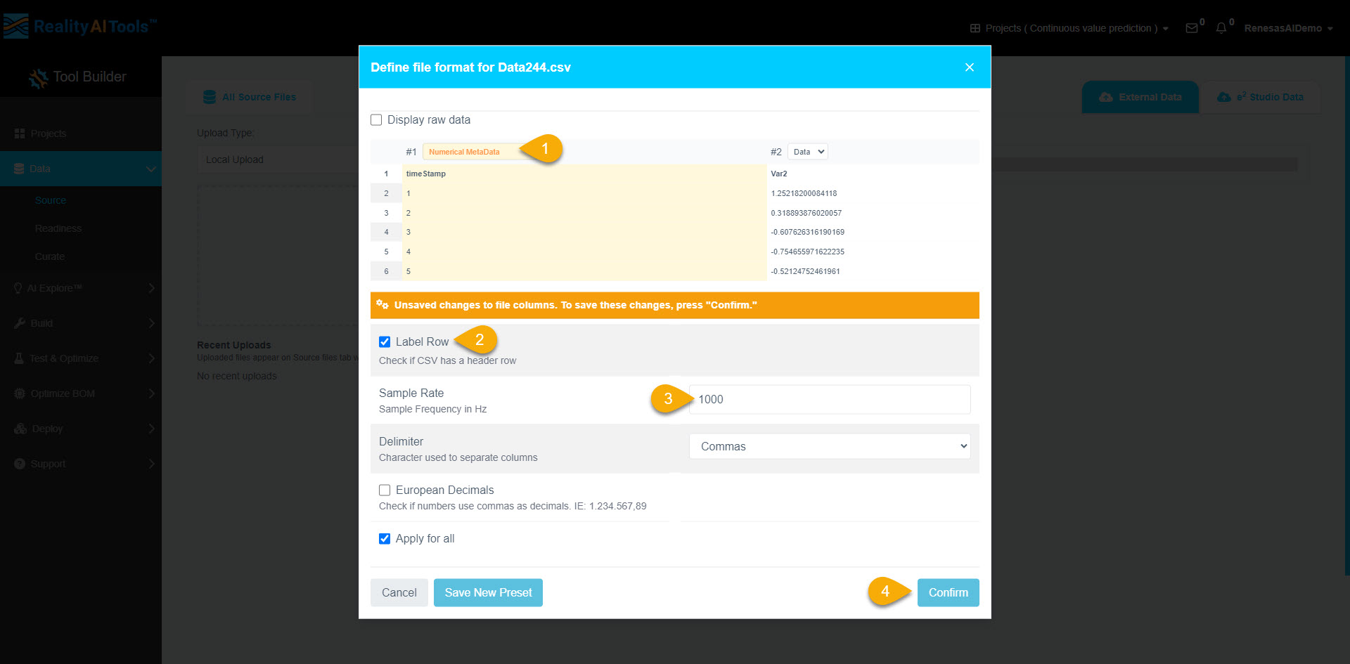
- Once uploaded, a formatting window will appear.
- Click Data > Numeric Metadata to label the first column of the dataset.
- Select the Label Row checkbox.
- Set the sample rate as 1000 Hz.
- Click Confirm to apply formatting to all files.
- The dataset is now uploaded and formatted successfully.
Step 2: Curating and Preprocessing Dataset
- Version 5.6.6
- Version 6.0
To prepare the dataset, break the data files into smaller segments. These segments serve as inputs for the machine learning (ML) model.
For example:
- If a data file is 10 seconds long, split it into ten 1-second segments.
- Adjust the segment length based on prior knowledge or experimentation.
- For this tutorial, use a 1-second window length.
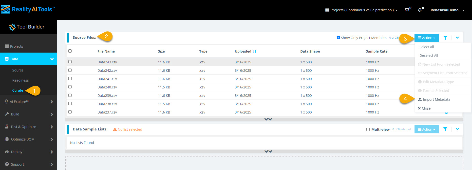
Step 2.1: Navigate to Curate Options and Import Metadata
- In the left menu, select Data > Curate.
- Select the Source Files tab to expand the section.
- Select Action > Import Metadata to assign labels (Ground Truths) to the data files.
- Select the file upload space to open the file explorer.
- Select metadata.csv from the dataset directory.
Step 2.2: Assign Target Value Labels
- Set the first dropdown to File Names.
- Set the second dropdown to Target Value to label the files correctly.
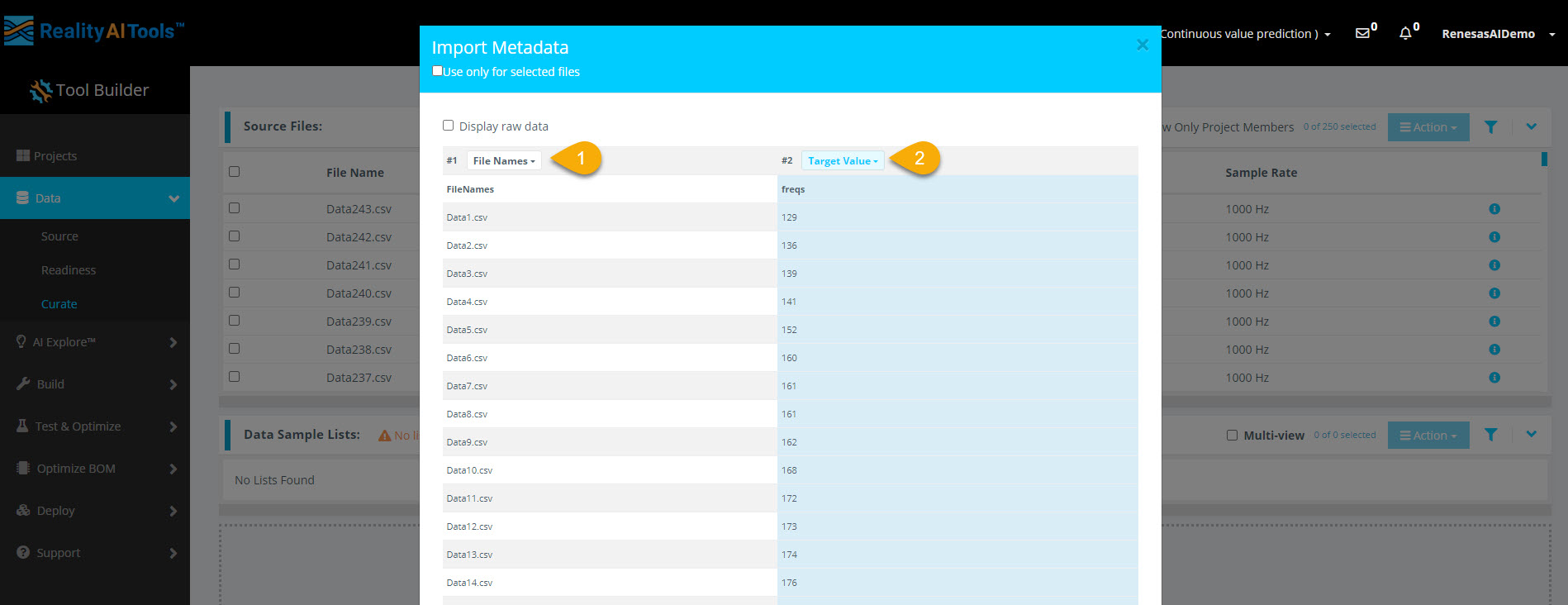
Why Use Target Value?
- Target Value represents labels for continuous value (regression) problems in ML.
- The model recognizes only Target Class or Target Value for labeling and Data for sensor readings.
- Other metadata like time, date, and numeric values help with sorting but do not affect model training.
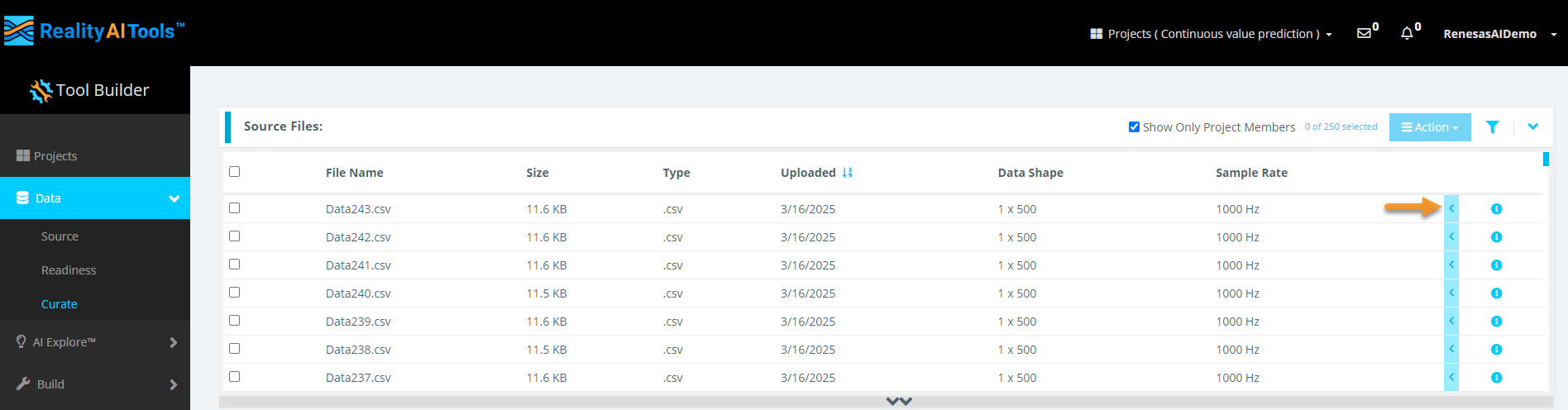
Step 2.3: Verify Assigned Labels
- Select the blue arrow next to a file name to view the assigned labels.
Step 2.4: Select Files for Segmentation
- Select Action > Select All to choose all files.
- Select Action > Segment List from Selected to open the segmentation window.
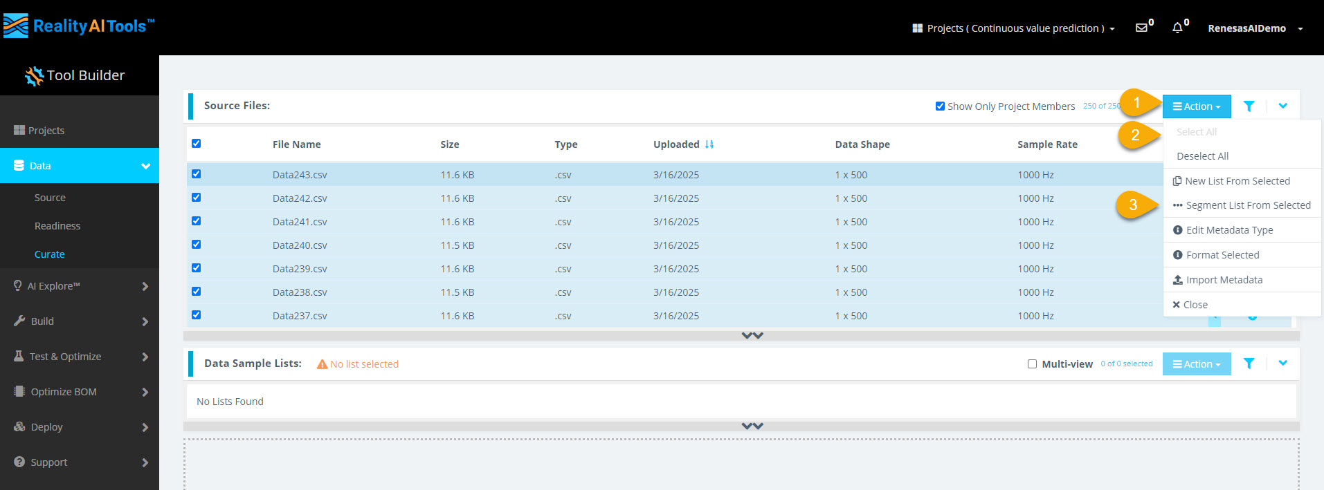
Why Segment the Data?
- ML models on Renesas MCUs operate in resource-constrained environments.
- They must process live data efficiently in small time windows (e.g., 1 sec, 500 ms).
- Instead of analyzing long data streams, breaking data into smaller segments helps the model adapt to real-world conditions.
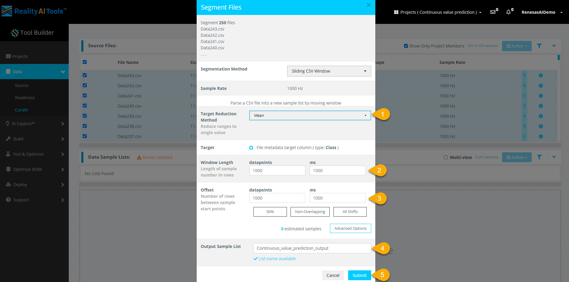
Step 2.5: Configure Segmentation Parameters
In the segmentation window, enter the following details:
- Target Reduction Method:
Mean - Window Length:
1000 milliseconds(1 sec) - Offset:
1000 milliseconds(1 sec)
After entering the parameters:
- Enter a name in the Output Sample List field.
- Select Submit to start segmentation.
Here,
- Window Length: Defines how much data the model analyzes for classification.
- Offset: Sets the gap before creating the next segment.
- A 50% overlap balances data variation and redundancy.
- Non-overlapping windows work best with large datasets.
- Offset = 1 (All Shifts) is useful for testing after selecting a classifier.
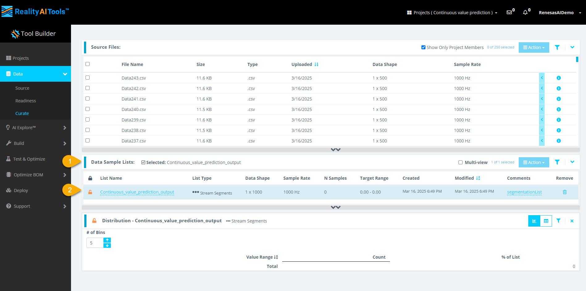
Step 2.6: View Processed Data
- Wait ~30 seconds, then refresh the page.
- Select the Data Sample List tab to view the processed segments.
- Select a sample to Curate and analyze its histogram.
- The segmentation process takes less than 1 minute for small datasets.
- Larger files (e.g., 1 GB) may take 5-10 minutes to segment.
- If the histogram does not appear immediately, refresh the page.
- The dataset is now curated and preprocessed successfully.
Overview
In this section, we will:
- Inference Target assign inference target.
- Create Dataset organize the files into a dataset.
- Break down data files into smaller segments.
- Prepare the dataset for Machine Learning (ML) model training.
🔹 Why segmentation?
- Machine Learning models process small, time-based segments for predictions.
- If a data file is 10 seconds long, we can split it into 1-second segments (10 total).
- This helps the model analyze and classify real-time data efficiently.
For this tutorial, we will use a 1-second window length.
Step 2.1: Access the Curate Section and Project Files
- Navigate to Data > Curate on the left navigation menu.
You will see the uploaded data set with sample rate applied.
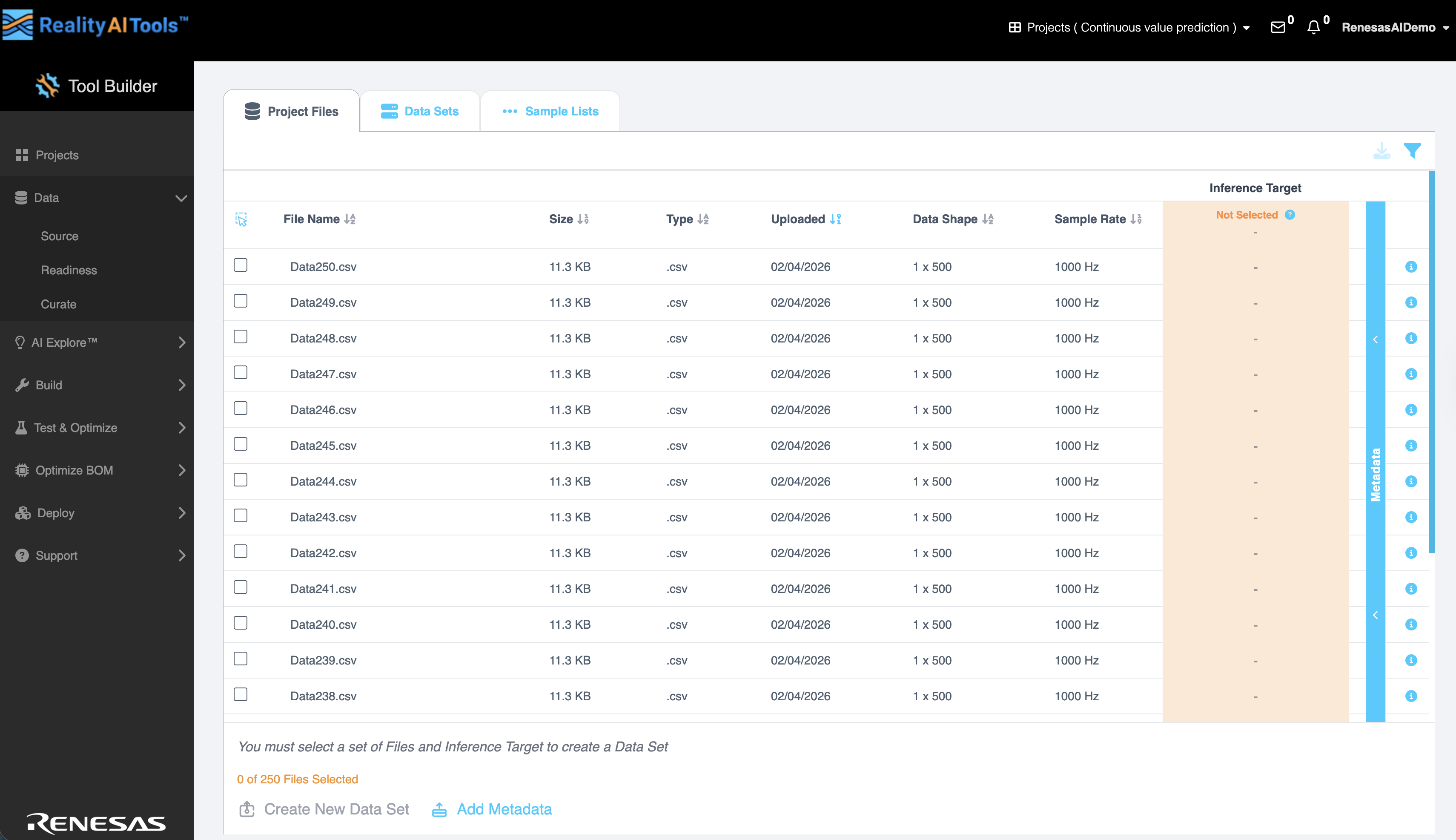
- Click Add Metadata at the bottom of the page to upload the metadata file.
Step 2.2: Create new dataset
- Select all files and click on the blue Metadata line on the right.
- Click on the downward arrow and select Target Class. This will select the Class column as the Inference Target. This utility is especially needed if you have multiple classes in the dataset and want to switch between classes when analyzing the dataset.
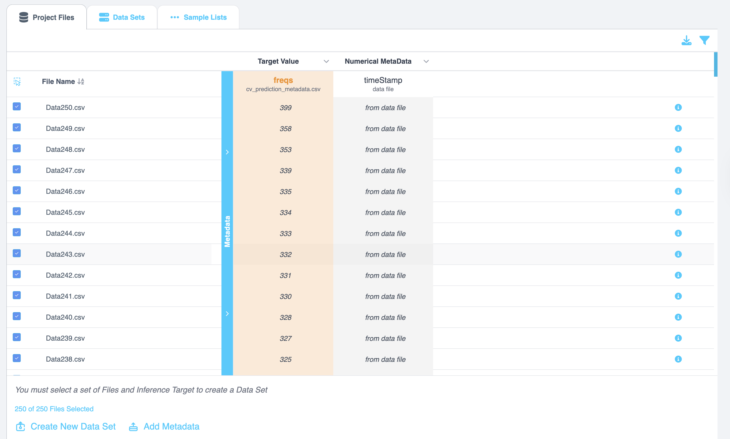
- You will see that the Inference Target section now says Target Class
- Select All Files
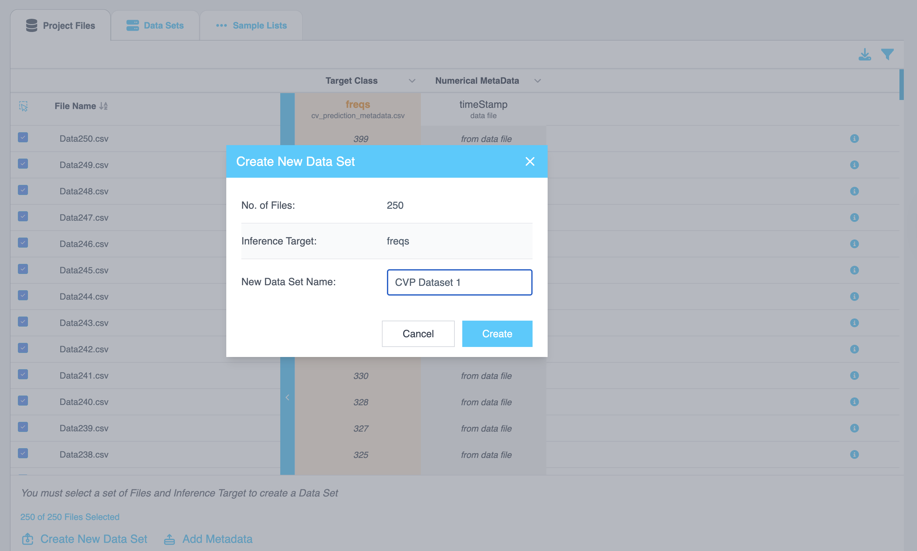
- Click on Create New Dataset. This action will organize the files into a list/ data set. This feature is especially helpful if you have huge amount of data (> 500 files). Organizing files across, days, months, metadata types, etc is valuable.
- Once a menu pops open, give the data set a name and click Create.
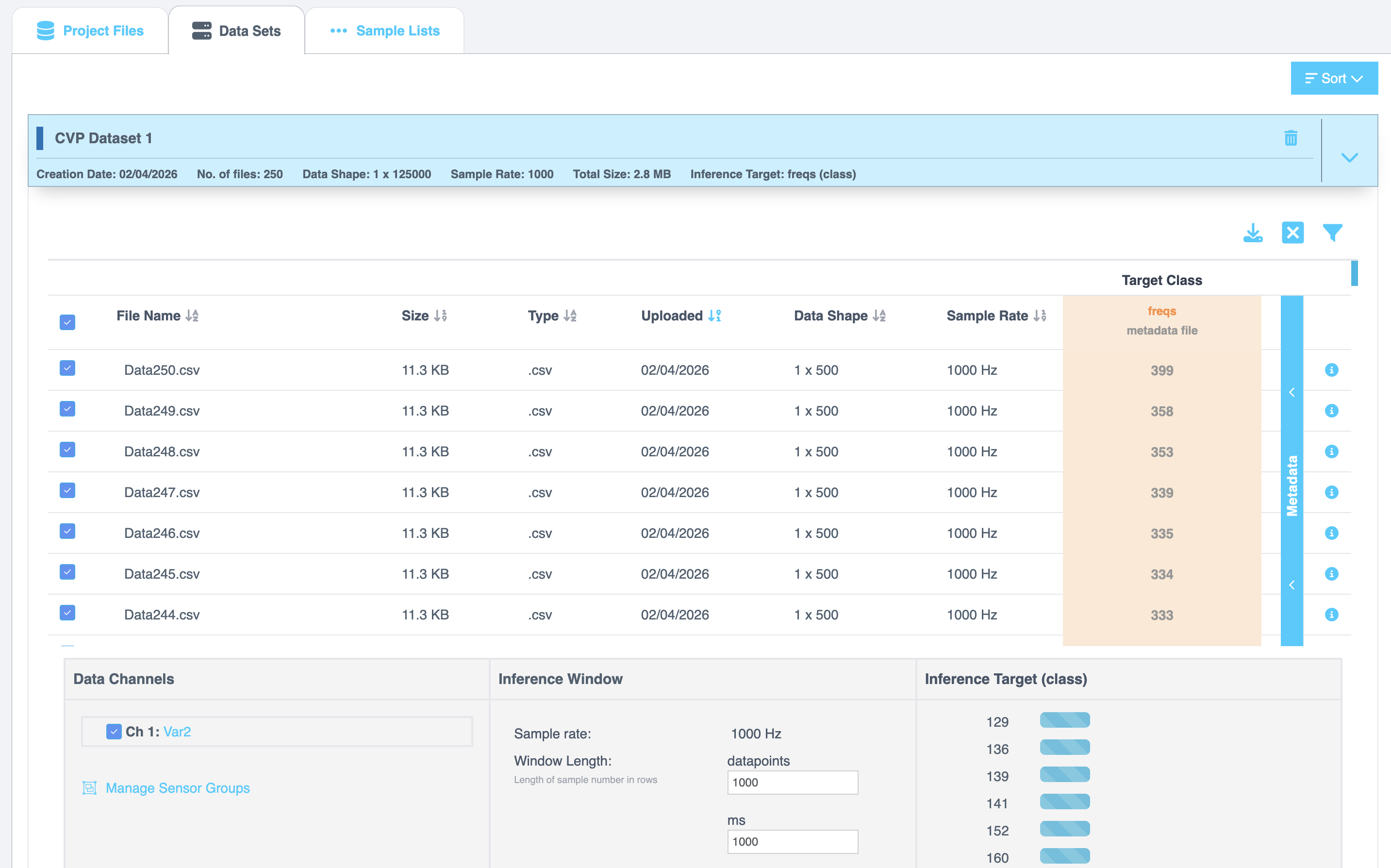
Step 2.2: Select Data sets for Segmentation and Configure Parameters
- Click on Data Sets tab at the top and further select the Data set we just created.
- Once you have expanded the data set, we will create a sample list. Sample list is just a collection of blocks/ pieces/ buffers of data files. We will use 1 second as window/ buffer/ block length for this tutorial. Navigate to the bottom and click on Create Sample List.
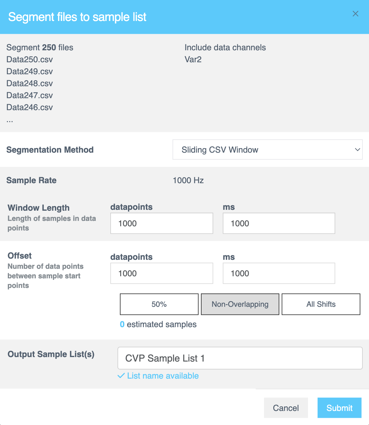
- You can create a single list or use random splits to divide the files into train,test,...and more. For simplicity, we will just go with single list.
- Assign the Window Length as 1 second and select Non-Overlapping as option for the windows/ blocks of data. Click Submit after.
- Window Length:
1000 ms(1 second) - Offset:
1000 ms(non-overlapping segments) - Segment Name: Enter a meaningful name
 Why segment data?
 - Real-time ML models deployed on Renesas MCUs must process live data efficiently.
- Shorter time windows (e.g., 1 second or 500 ms) allow quick predictions.
- Breaking down raw training data mimics real-world, real-time conditions.
Additional Information:
- Window Length: Defines how much data is considered in one classification.
- Offset: Controls how far the parser moves before creating a new segment.
50% overlap(offset = half of window length) is a good balance.Offset = 1(all shifts) is useful for final testing to simulate real-world performance.No overlapis better when data is abundant.
Step 2.4: Verify Segmentation and View Segmented Data
- Navigate to Samples List tab.
- Wait for ~30 seconds (varies based on dataset size).
- Refresh the page if needed and navigate to the tab.
- Click on the finished list and expand to see the histogram.
- Segmenting this dataset takes less than 1 min.
- Larger files (e.g., 1 GB) may take 5-10 minutes.
You have successfully:
- Segmented the dataset into 1-second blocks
- Created structured input for the ML model
Step 3: Analyzing Data and Creating Initial Models
In this section, you will create AI models using the uploaded dataset and analyze various statistics for those models.
Step 3.1: Create Initial Models
- In the left menu, click AI Explore.
- Click Values and RUL.
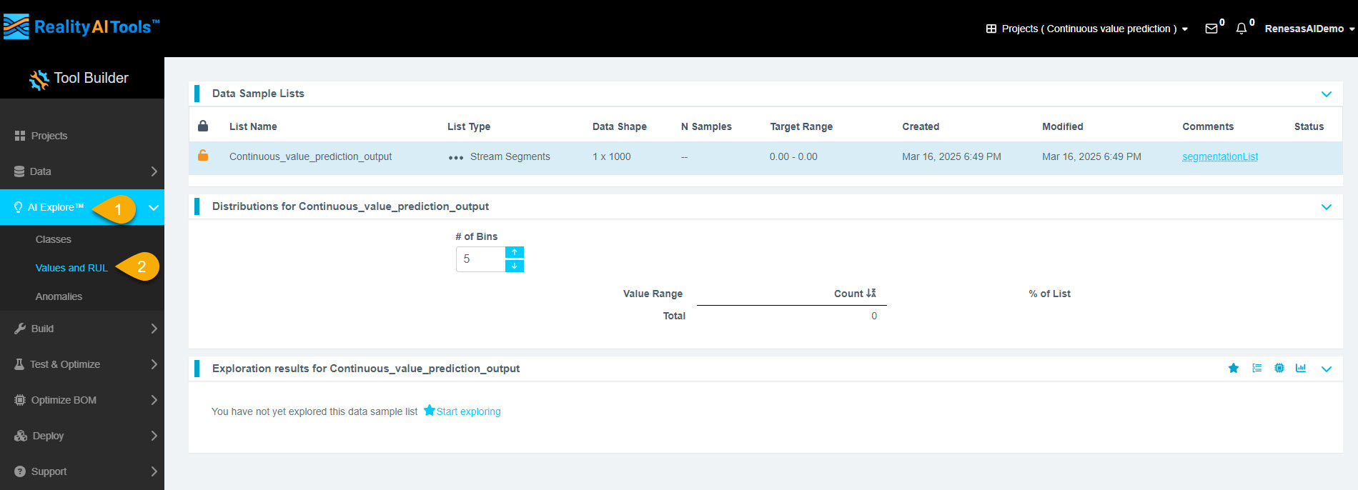
Step 3.2: Choose the AI Model Type
Reality AI Tools provides three types of AI models:
- Classes: Use when you have labeled categorical data. This is for classification models that use supervised learning.
- Values: Use when your dataset contains discrete integer or float values instead of categories. Examples include machine temperature or tire pressure. This is also supervised learning. (This tutorial uses this option.)
- Anomalies: Use for anomaly detection. This is a semi-supervised model that requires only normal data to create a baseline model.
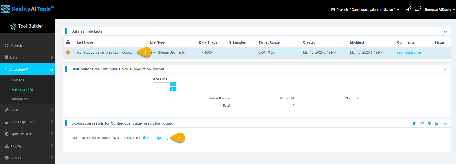
Click the segmented list once you are on the Classes page.
Step 3.3: Start Model Exploration
- Click the list.
- Click Start Exploring to generate models.
Step 3.4: Monitor Model Generation Progress
You will see the progress of the model generation process.
What Happens in the Background?
- Clicking Start Exploring triggers the Reality AI algorithm to analyze your data.
- The algorithm creates optimized feature sets and machine learning models that best fit the classification problem.
- It displays the best-performing models.
How the Algorithm Works
- AI Explore finds the best feature sets and machine learning parameters.
- Promising feature sets are used to construct machine learning models.
- Models are trained on a sub-sample and validated using K-Fold validation.
- Only the top-performing models are displayed.
What is K-Fold Validation?
K-Fold validation splits a dataset into K sections. Each section is used as a testing set once, while the remaining sections train the model.
For example, in 10-Fold validation (K=10):
- The dataset is split into 10 folds.
- In each iteration, one fold is the test set, and the remaining folds train the model.
- This process repeats until all folds have been used as test sets.
AI Explore uses K=10 for model evaluation.
Step 3.5: View Model Performance
As the system explores feature spaces, the top-performing models appear on the page.
Step 3.6: Analyze Model Results
- In the Exploration Results section, each row represents a different model based on features identified during AI Explore.
- Click Confusion Matrix to view detailed accuracy statistics.
Step 3.7: View Confusion Matrix and Regression Plot
- The Confusion Matrix/Regression Plot pop-up appears.
- Click the second option at the bottom for detailed statistics.
Note:
- The first option shows a confusion matrix with overall accuracy and error distribution.
Step 3.8: Analyze Error Distribution
The error distribution plot helps visualize error concentration across the numeric range.
- A wider distribution indicates poor model performance.
- The Regression Plot (Actual vs. Predicted) for the first model appears at the top.
- The sample-wise residual errors plot appears below.
What is Residual Error?
A residual is the vertical distance between an observed data point and the regression line. It represents the prediction error.
What is R²?
R-squared (R²) measures how well a regression model explains the variation in the dependent variable.
What is MAE?
Mean Absolute Error (MAE) is the average of absolute errors in predictions.
Step 3.9: View Resource Consumption
Hover over the complexity tab to view estimated resource consumption.
Understanding Complexity Numbers:
- X operations: Multiplication operations required for the model.
- Feature Space: Operations needed for feature calculations.
- Classifier: Operations required for predictions. (This is blank for regression models.)
- Total: Sum of all operations.
Step 3.10: Interpret Complexity Numbers
- Complexity numbers estimate resource consumption on the MCU/MPU.
- They are not final and can be optimized.
- Example: If a model focuses on frequency bands less than 50 Hz, filtering out unnecessary data can reduce resource use.
- If a target processor was preselected, top models will fit within its resource limits.
Step 3.11: Deploy the Model
After reviewing the statistics:
Click Deploy Model for further testing and export.
Step 3.12: Name and Save the Model
- Enter a name for the exported model.
- Click Add.
Step 3.13: Verify Deployment
- The deployed model's icon changes to indicate success.
- Hover over the icon to view the model name.
- If the deployment fails, contact customer support.
You have successfully completed this section.
Step 4: Testing the Model
In this section, we will test a trained model using sample data, analyze the results, and export the findings.
Step 4.1: Navigate to the Test Section
- In the left menu, click Test & Optimize and then Try New Data.
- This section allows you to test models with new datasets.
Step 4.2: Select Model and Data Sample List
- Choose the trained model (referred to as Trained Tool) and select the Data Sample List you want to test.
- Click the Accuracy Test button to start a test job.
Note:
- To test the model on a blind dataset, you must upload and segment the data (see Sections 1 & 2).
- In this tutorial, we will test the model against the same dataset used for training.
Step 4.3: Wait for Test Job Completion
- After triggering the test, wait 2–3 minutes and refresh the page.
- Click the Trial Results tab to view the results.
Note:
- The test duration varies based on dataset size.
- A 1 GB dataset may take approximately 10 minutes to complete.
Step 4.4: View Regression Plot
- Click the second option button (highlighted in the UI) to view the Regression Plot.
- Refer to Section 3.8 for details on interpreting these plots.
Step 4.5: Review Test Statistics
- The statistics will be displayed in a format similar to AI Explore results.
- If the test data includes labeled values, a Regression Plot will be generated.
- If no labeled data is provided, no plot will be produced, but you can still export raw results.
Step 4.6: Export Results
- Click Show Sample Level Details (bottom left) to review detailed test data.
- To export the results, click Export to CSV.
Step 4.7: Understanding the Results
- Results: Predictions made by the Reality AI algorithm.
- Expected Results: Ground truth labels assigned during data upload.
Note:
- You can filter the view to display only correct or incorrect results.
- To analyze waveform data for each segment, go to the View Sample tab.
- This helps compare successful vs. unsuccessful predictions.
You have successfully completed this section.