Fan condition monitoring
Introduction
This tutorial provides a step-by-step guide to using Reality AI Tools portal from Renesas to build AI models for non-visual sensing applications. We will work with a vibration dataset collected using a 3-axis accelerometer to identify different conditions of a fan stack.
Objectives
By the end of this tutorial, you will:
- Gain hands-on experience using Reality AI Tools with a vibration dataset.
- Learn how to analyze and build ML models for non-visual sensing applications.
Requirements
Before starting, ensure you have the following:
Hardware & Software
- A PC or MacBook with Chrome or Firefox installed.
Dataset
- 21 CSV files containing vibration data collected from a 3-axis accelerometer.
- Download dataset here: Fan condition monitoring
Estimated Time
90 minutes
Step 1: Creating a Project and Uploading a Dataset
Overview
In this section, we will:
- Set up a new project on Reality AI Tools
- Upload and format the dataset
Step 1.1: Unzip the Tutorial Data
- Locate the TutorialData.zip file.
- Extract the contents.
- Verify that the folder contains 21 CSV files.
Step 1.2: Access Reality AI Tools Portal
- Open your browser (Chrome or Firefox recommended).
- Navigate to portal.reality.ai.
- Enter your login credentials (provided via email).
- Click Login.
Step 1.3: Create a New Project
- After logging in, you will see the portal dashboard.
- Click Add Project to create a new project.
- Fill in the project details:
- Project Name: Enter a meaningful name.
- Description (Optional).
- Click Add Project.
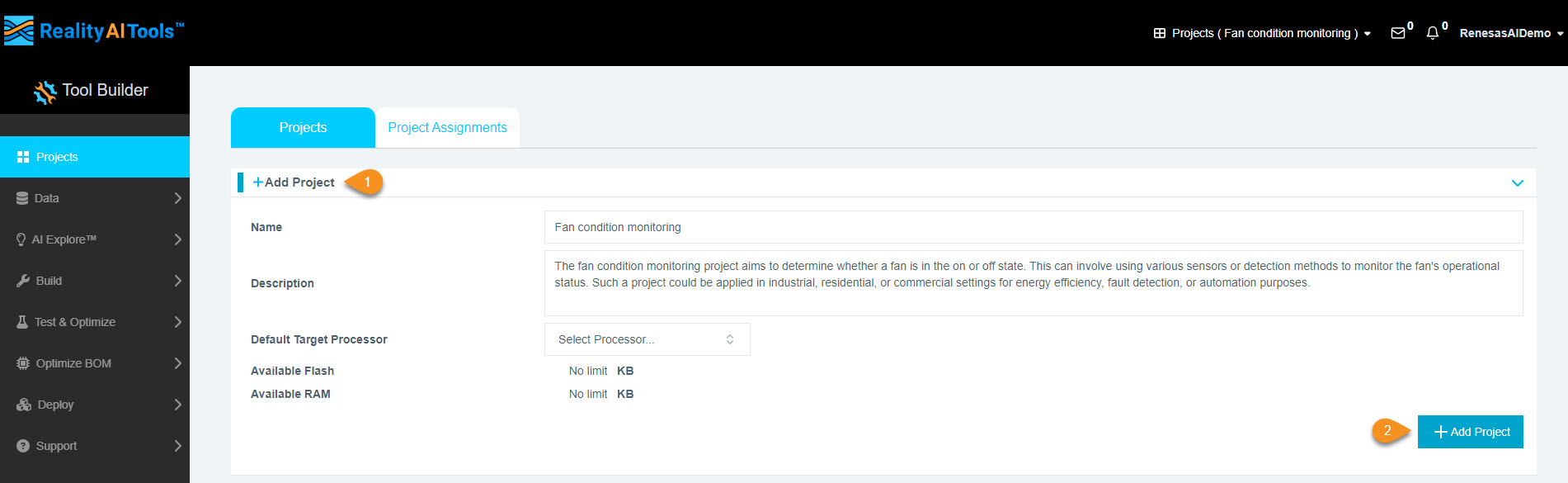
Why create a project?
A project will store your dataset and all subsequent analysis.
Step 1.4: Select the Project
- Click the newly created project tab.
- This will open the project and allow you to perform various functions.
Step 1.5: Upload Dataset
- In the left menu, click Data > Source.
- Click Drop file here to upload files.
- Navigate to the TutorialData folder.
- Select all 21 CSV files and click Open.
- The upload progress will be displayed on the screen.

Step 1.6: Format the Uploaded Data
After the upload is complete, a formatting page will appear.
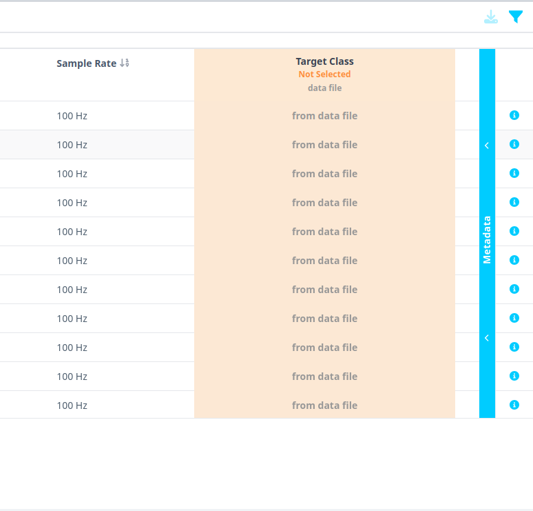
- Click the Data dropdown and select Target Class.
- Check the Label Row box.
- Assign Sample Rate =
100Hz. - Click Confirm to finalize formatting.
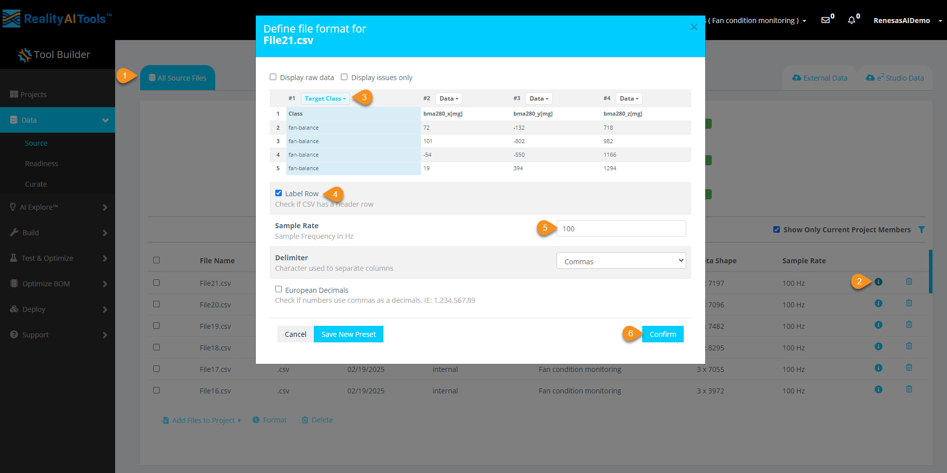
What is Target Class?
- It represents labels for classification problems in Machine Learning.
- In this case, it classifies different fan conditions:
- Fan-On, Fan-Off, etc.
- If dealing with numerical values (e.g., temperature), we would use Target Value instead.
Other options in the dropdown?
- Target Class: Categorical labels (e.g., Fan state).
- Target Value: Numerical labels (e.g., sensor readings).
- Data: Raw sensor data used for model training.
- Other fields like Time, Date, Metadata are useful for sorting but do not impact model training.
Step 2: Curating and Preprocessing the Dataset
- Version 5.6.6
- Version 6.0
Overview
In this section, we will:
- Break down data files into smaller segments.
- Prepare the dataset for Machine Learning (ML) model training.
🔹 Why segmentation?
- Machine Learning models process small, time-based segments for predictions.
- If a data file is 10 seconds long, we can split it into 1-second segments (10 total).
- This helps the model analyze and classify real-time data efficiently.
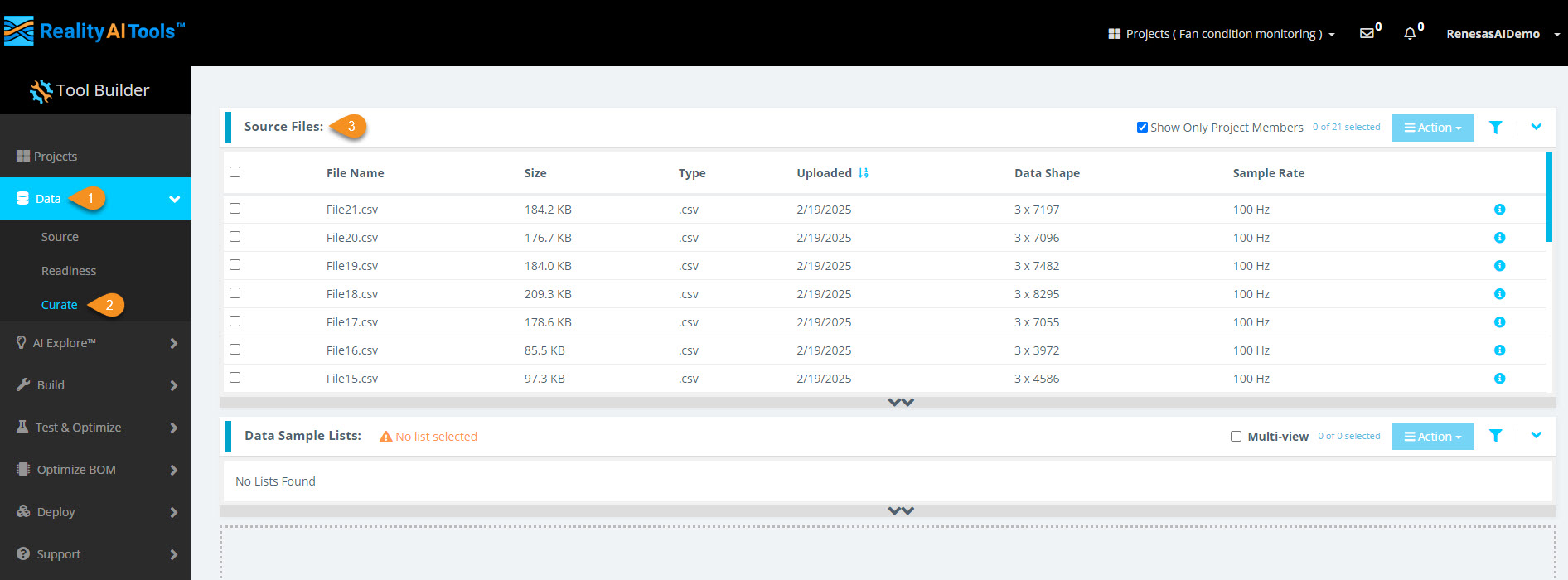
Step 2.1: Access the Curate Section and Upload Data
- In the left menu, click Data > Curate.
- Click the Source Files tab to expand it.
- You will see all uploaded CSV files.
Step 2.2: Select All Files for Segmentation
- Click the Select All checkbox to select all CSV files for segmentation.
- Click the Action button.
- Click Segment List from Selected to open the segmentation window.
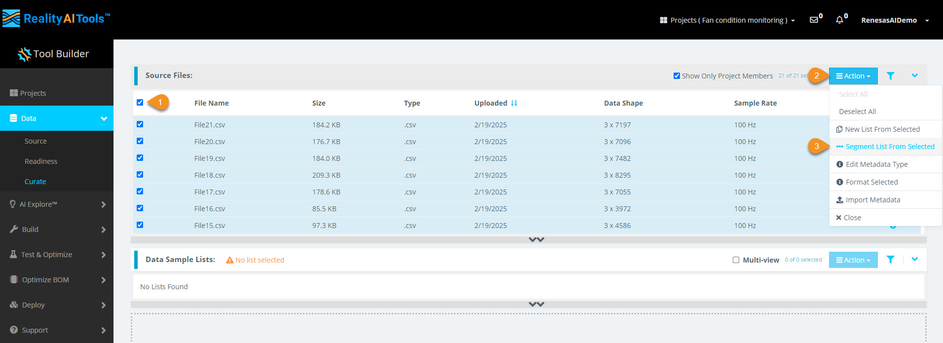 Why segment data?
- Real-time ML models deployed on Renesas MCUs must process live data efficiently.
- Shorter time windows (e.g., 1 second or 500 ms) allow quick predictions.
- Breaking down raw training data mimics real-world, real-time conditions.
Step 2.3: Configure Segmentation Parameters
Once the segmentation window appears, enter the following:
- Window Length:
100 ms(0.1 second) - Offset:
100 ms(non-overlapping segments) - Segment Name: Enter a meaningful name
Click Submit to begin segmentation.
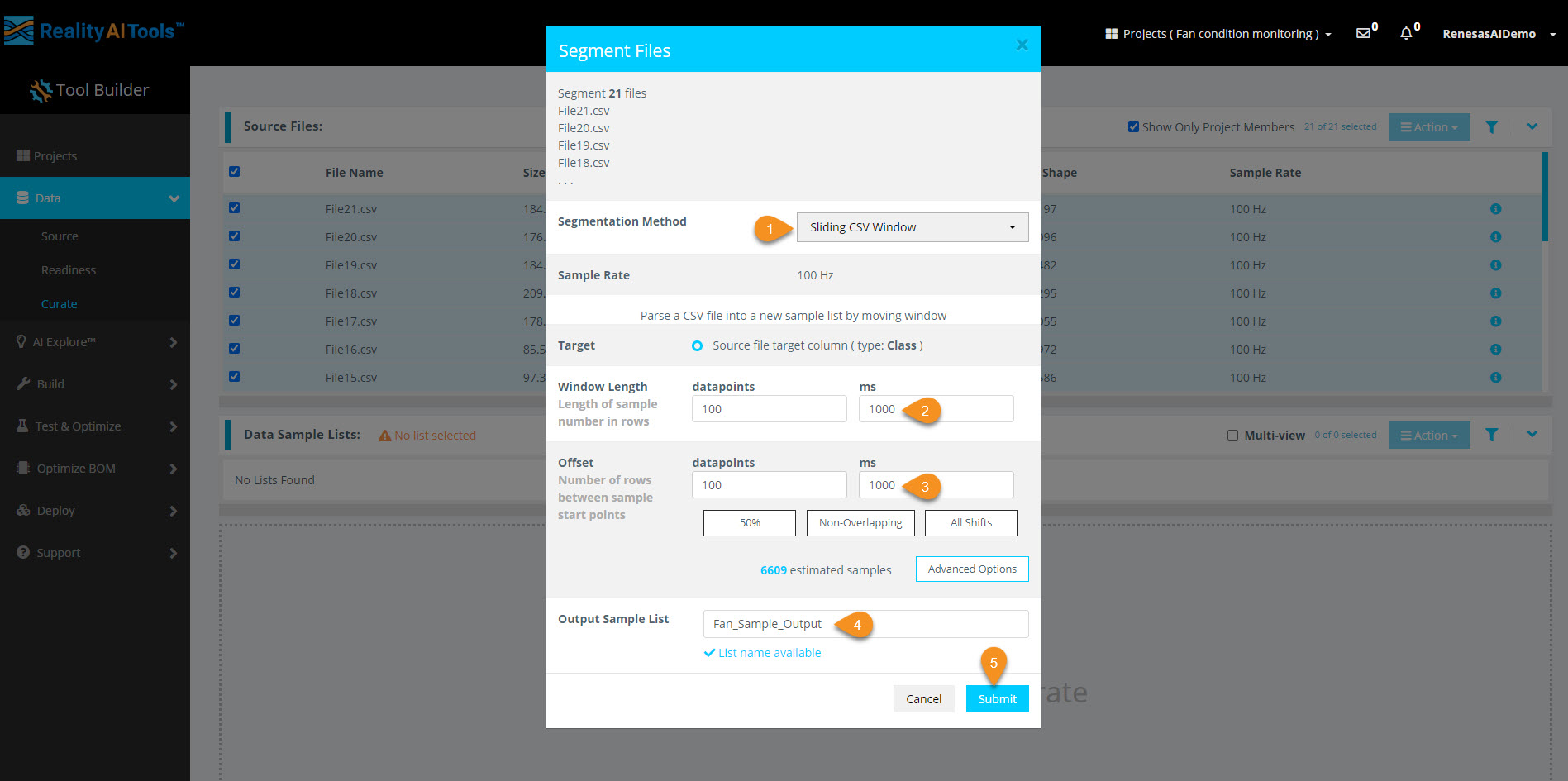 Additional Information:
- Window Length: Defines how much data is considered in one classification.
- Offset: Controls how far the parser moves before creating a new segment.
50% overlap(offset = half of window length) is a good balance.Offset = 1(all shifts) is useful for final testing to simulate real-world performance.No overlapis better when data is abundant.
Step 2.4: Verify Segmentation
- Wait for ~30 seconds (varies based on dataset size).
- Refresh the page.
- Click the Data Sample List tab.
- You should see the processed list of segmented data.
- Segmenting this dataset takes less than 1 min.
- Larger files (e.g., 1 GB) may take 5-10 minutes.
Step 2.5: View Segmented Data
- Click anywhere on the new segmented list.
- A histogram of the segmented data should appear.
- If the histogram does not load, refresh the page.
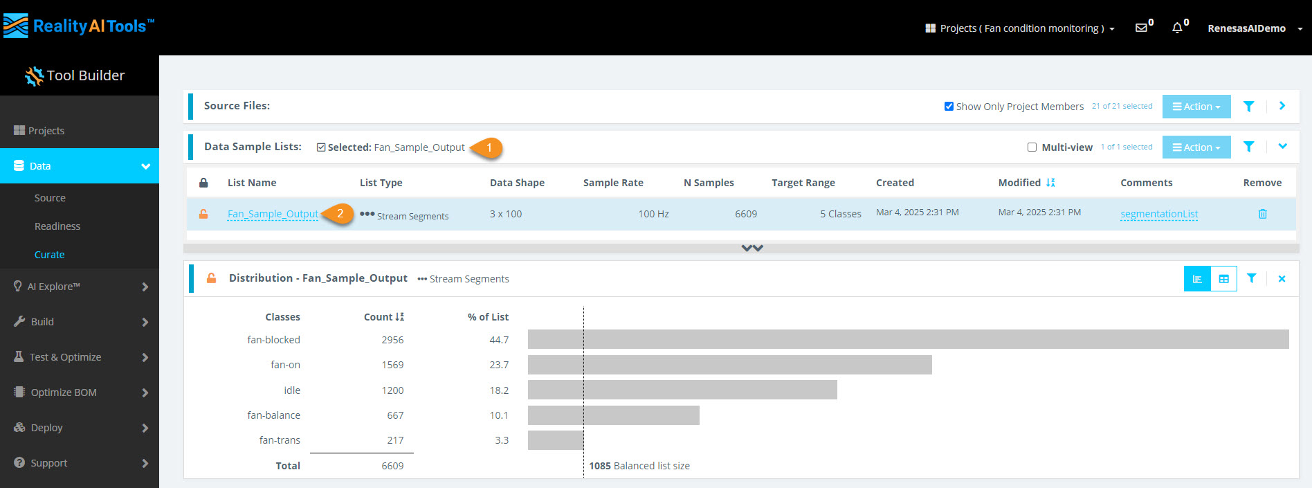
You have successfully:
- Segmented the dataset into 1-second blocks
- Created structured input for the ML model
Overview
In this section, we will:
- Inference Target assign inference target.
- Create Dataset organize the files into a dataset.
- Break down data files into smaller segments.
- Prepare the dataset for Machine Learning (ML) model training.
🔹 Why segmentation?
- Machine Learning models process small, time-based segments for predictions.
- If a data file is 10 seconds long, we can split it into 1-second segments (10 total).
- This helps the model analyze and classify real-time data efficiently.
Step 2.1: Access the Curate Section and Project Files
- Select all files and click on the blue Metadata line on the right.
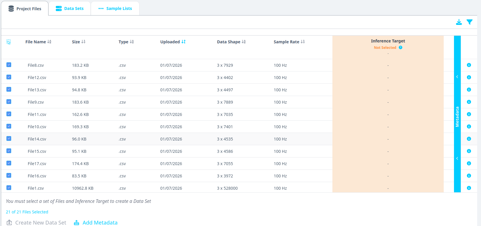
- Click on the downward arrow and select Target Class. This will select the Class column as the Inference Target. This utility is especially needed if you have multiple classes in the dataset and want to switch between classes when analyzing the dataset.
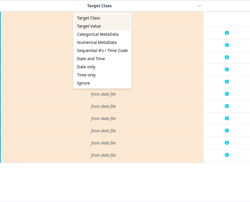
- You will see that the Inference Target section now says Target Class
- Select All Files
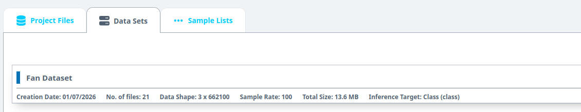
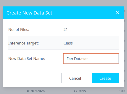
- Click on Create New Dataset. This action will organize the files into a list/ data set. This feature is especially helpful if you have huge amount of data (> 500 files). Organizing files across, days, months, metadata types, etc is valuable.
- Once a menu pops open, give the data set a name and click Create.
Step 2.2: Select Data sets for Segmentation and Configure Parameters
- Click on Data Sets option at the top and further select the Data set we just created
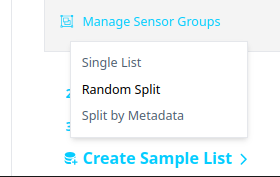
- Once you have expanded the data set, we will create a sample list. Sample list is just a collection of blocks/ pieces/ buffers of data files. Navigate to the bottom and click on Create Sample List.
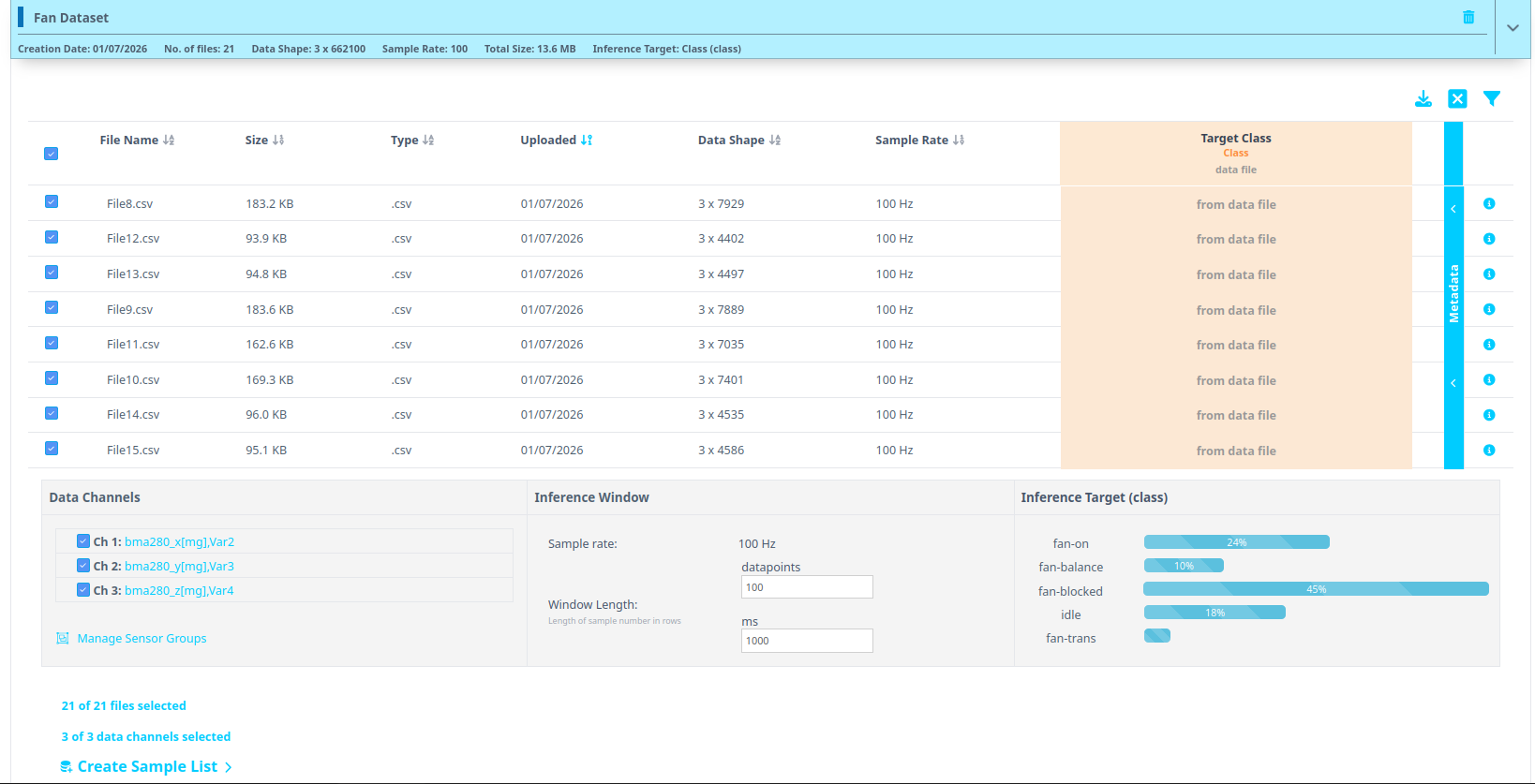
- You can create a single list or use random splits to divide the files into train,test,...and more. For simplicity, we will just go with single list.
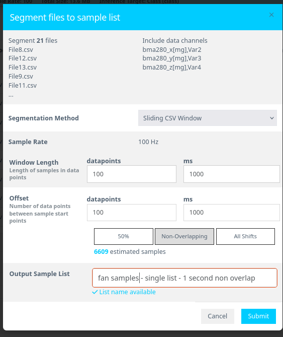
- Assign the Window Length as 0.1 second and select Non-Overlapping as option for the windows/ blocks of data. Click Submit after.
- Window Length:
100 ms(0.1 second) - Offset:
100 ms(non-overlapping segments) - Segment Name: Enter a meaningful name
Why segment data?
- Real-time ML models deployed on Renesas MCUs must process live data efficiently.
- Shorter time windows (e.g., 1 second or 500 ms) allow quick predictions.
- Breaking down raw training data mimics real-world, real-time conditions.
Additional Information:
- Window Length: Defines how much data is considered in one classification.
- Offset: Controls how far the parser moves before creating a new segment.
50% overlap(offset = half of window length) is a good balance.Offset = 1(all shifts) is useful for final testing to simulate real-world performance.No overlapis better when data is abundant.
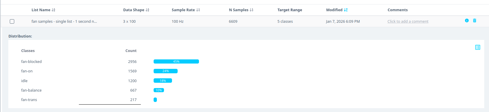
Step 2.4: Verify Segmentation and View Segmented Data
- Navigate to Samples List tab.
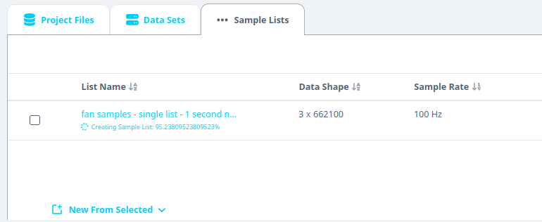
- Wait for ~30 seconds (varies based on dataset size).
- Refresh the page if needed and navigate to the tab.
- Click on the finished list and expand to see the histogram.
- Segmenting this dataset takes less than 1 min.
- Larger files (e.g., 1 GB) may take 5-10 minutes.
You have successfully:
- Segmented the dataset into 1-second blocks
- Created structured input for the ML model
Step 3: Analyzing Data and Creating Initial Models
In this section, we will create AI models using the uploaded dataset and analyze various statistics to evaluate model performance.
3.1 Accessing AI Model Creation
- On the left menu, click AI Explore, then select Classes.
3.2 Understanding AI Model Types
Reality AI Tools offer three types of AI models:
- Classes: Used for labeled categorical data (Supervised Learning).
- Example: Classifying objects into predefined categories.
- Values: Used for discrete integer or float values instead of categories (Supervised Learning).
- Example: Predicting temperature or tire pressure values.
- Anomalies: Used for anomaly detection (Semi-supervised Learning).
- Requires only normal data examples to create a baseline model.
Since we uploaded perfectly labeled data in Section 1, we will use the Classes option in this tutorial.
3.3 Creating Models
- Click the segmented list once you're on the Classes page.
- Click Start Exploring to generate AI models.
3.4 Understanding the Model Generation Process
After clicking Start Exploring, the Reality AI algorithm will:
- Create optimized feature sets and machine learning models.
- Identify the best-performing classification models.
- Display the most successful models.
3.5 Monitoring Model Progress
- As the system explores different feature spaces, you will see:
- The progress of model generation.
- A list of top-performing models.
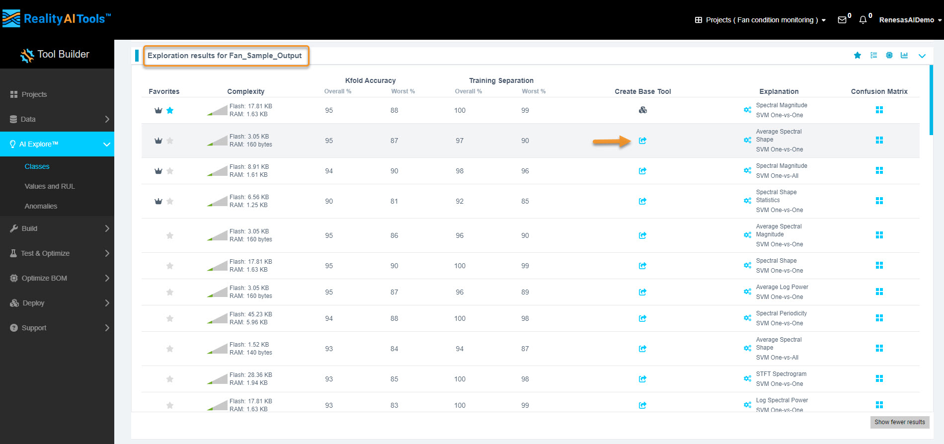
3.6 Viewing Exploration Results
- Each row in the Exploration Results section represents a different model based on unique feature sets.
- Click the Confusion Matrix option for detailed accuracy statistics.
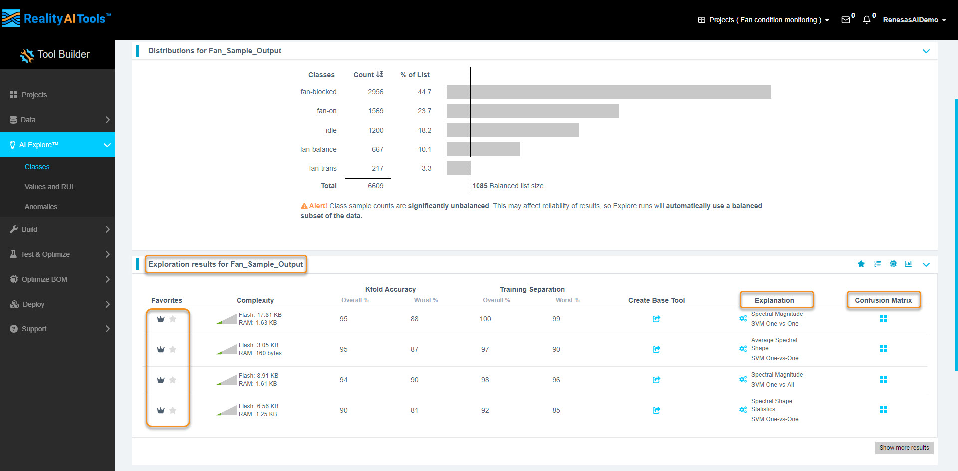
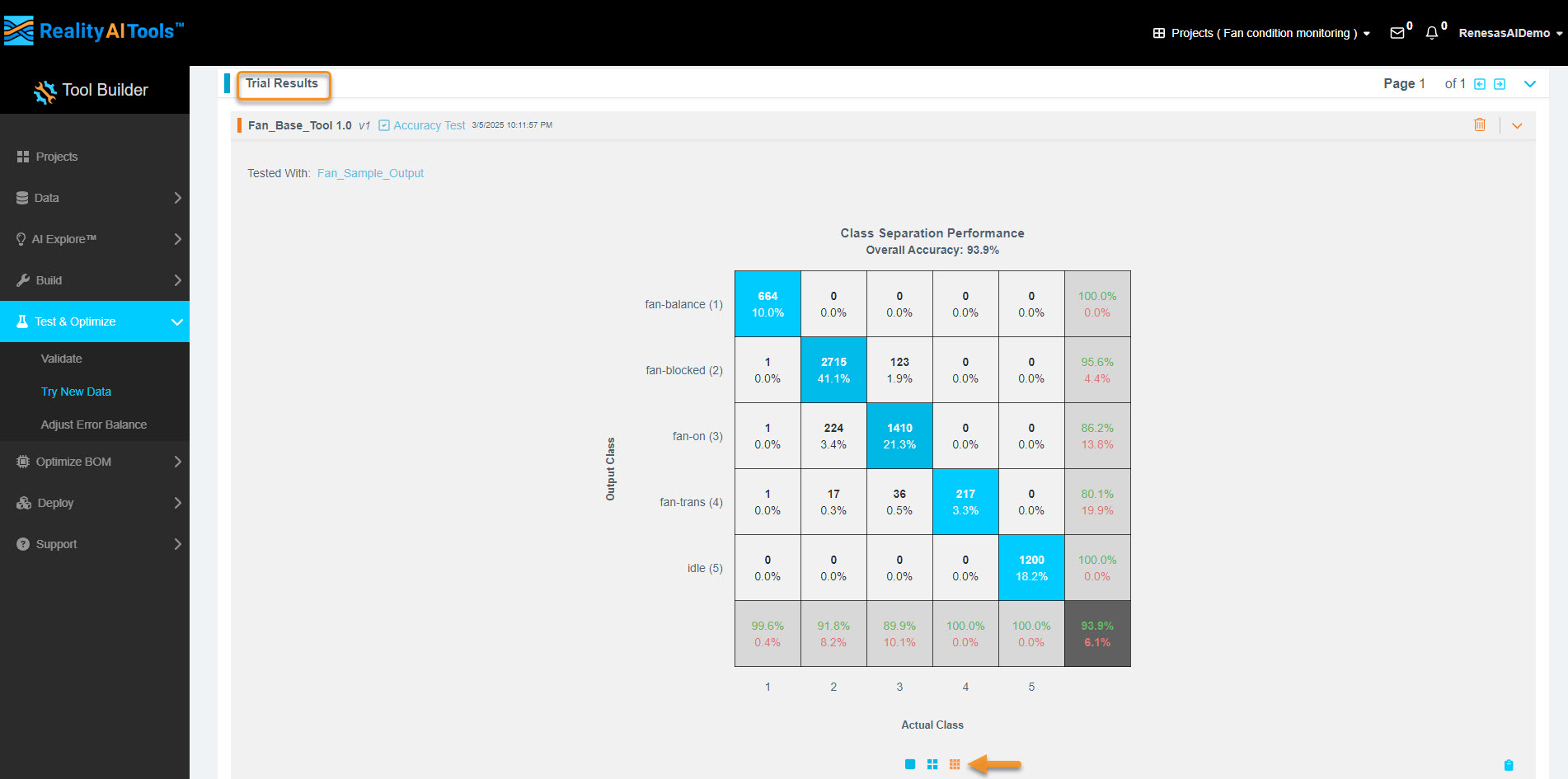
3.7 Understanding the Confusion Matrix
- Click the third option in the pop-up to expand detailed stats.
- Confusion Matrix Breakdown:
- Rows: Predicted class (model's output).
- Columns: Actual class (ground truth).
- Diagonal values (blue): True Positives & True Negatives.
- White cells: Misclassifications (False Positives & False Negatives).
- Bottom row:
- Green: Class accuracy.
- Red: Class error rate.
- Bottom-right corner: Overall accuracy (green) and error rate (red).
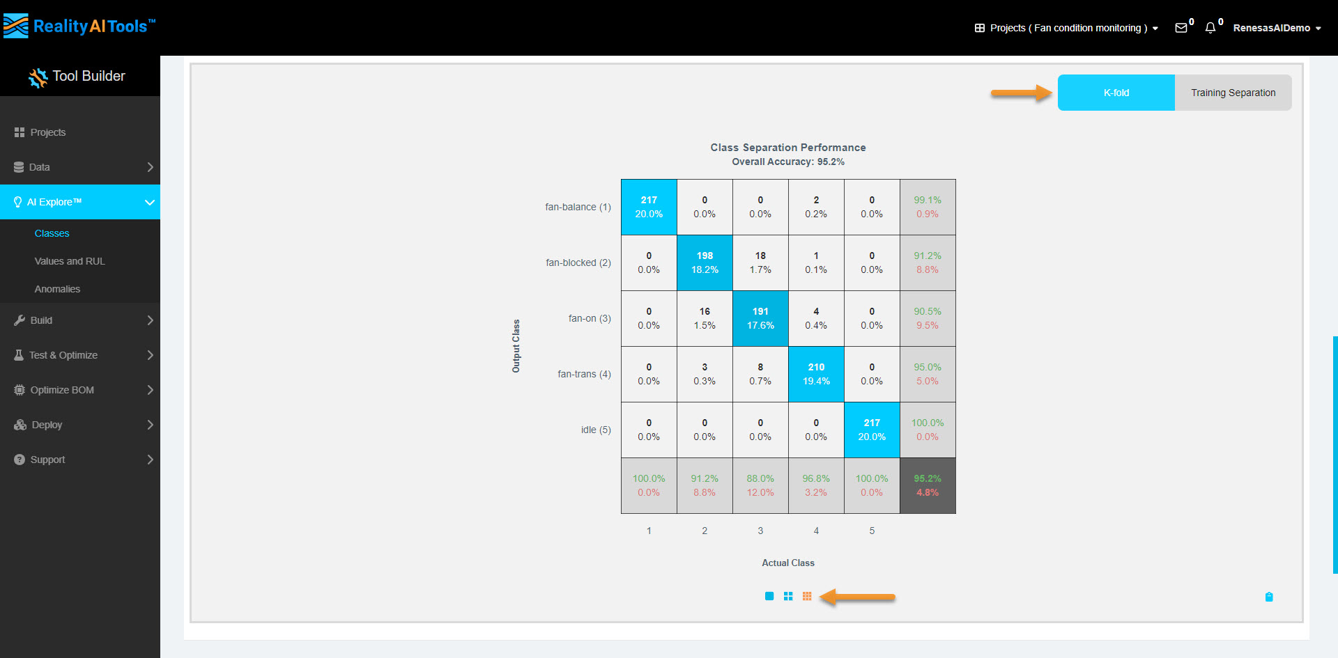
A good confusion matrix has minimal white cells (indicating fewer misclassifications).
3.8 Identifying Feature Space
- Click the Explanation tab.
- The feature space name (e.g., Spectral Shape) will pop up.
- Click the button to see detailed plots.
Interpreting Feature Space Plots
- Bottom Plot (Decision Significance):
- Shows the importance of frequency bands in classification.
- Low importance: Light blue, lower on Y-axis.
- Moderate importance: Dark blue, middle of Y-axis.
- High importance: Orange, high on Y-axis.
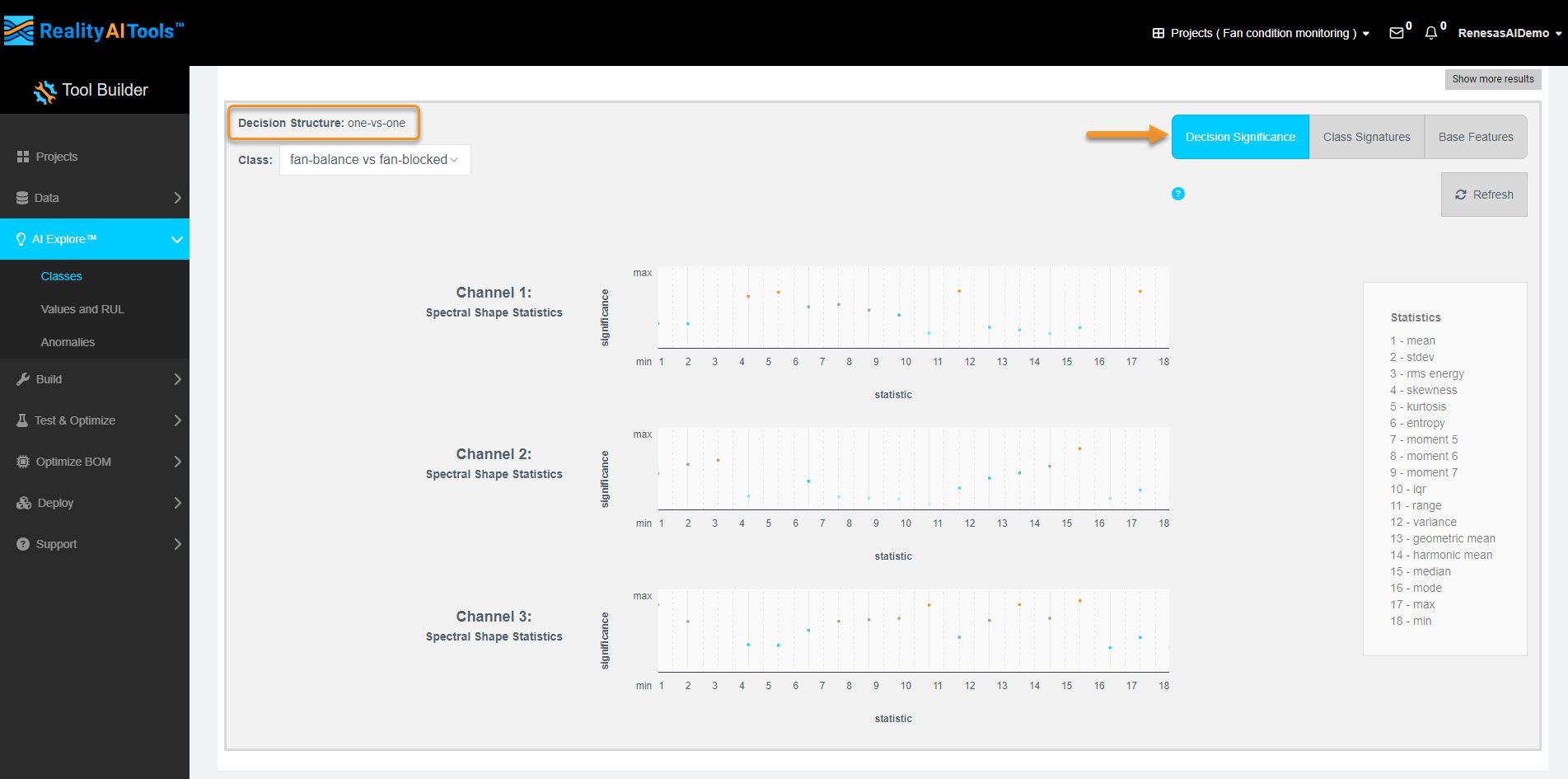
- Top Plot:
- Solid lines: Mean of signal.
- Dotted lines: Standard deviation of signal.
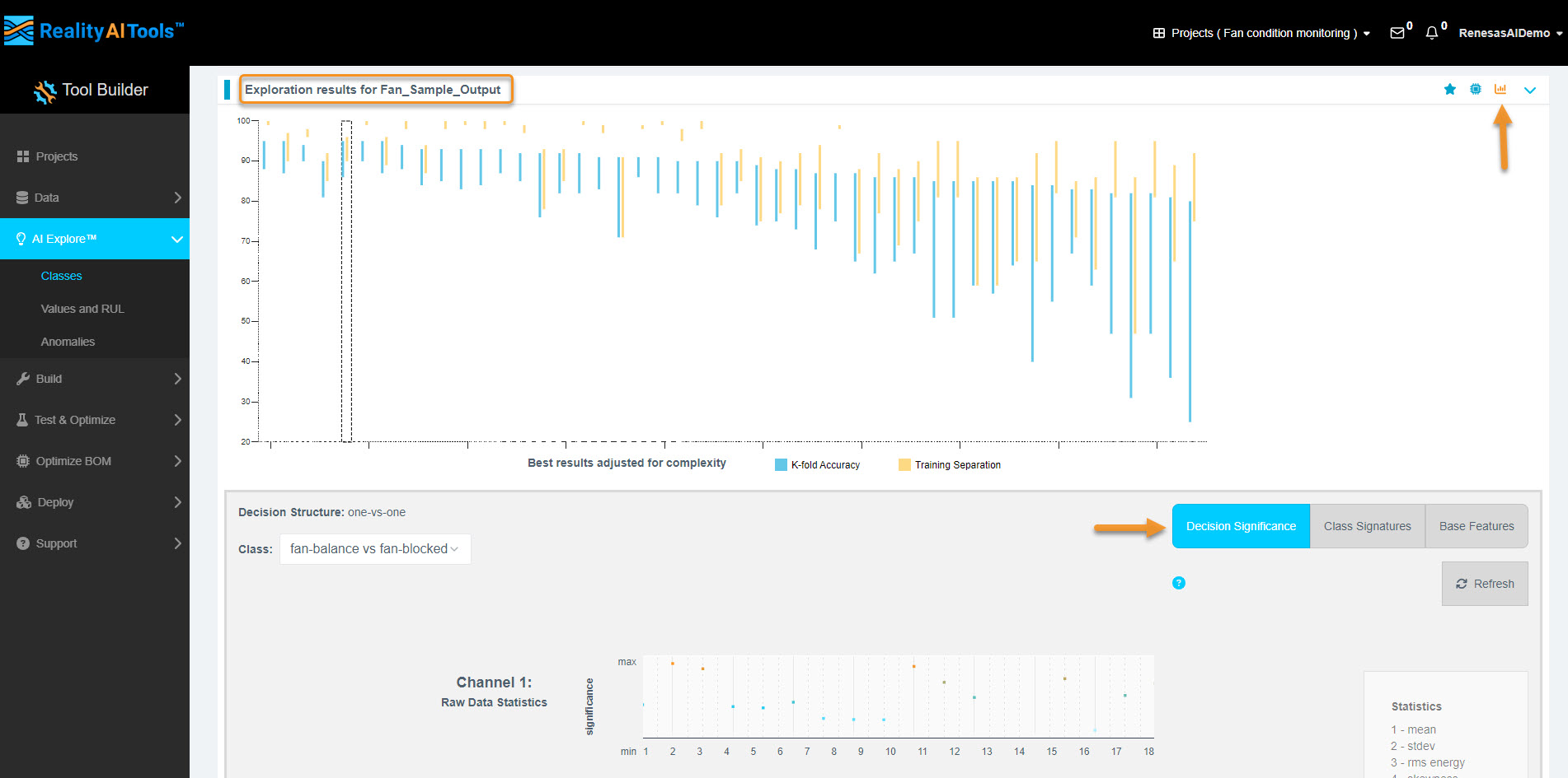
3.9 Assessing Model Complexity
- Hover over the Complexity tab to view resource consumption details.
- Interpretation of complexity numbers:
- Helps estimate computational resource requirements (MCU/MPU).
- Not final; further optimization is possible.
Optimization Tip:
If the decision significance plot shows key frequencies below 50 Hz, applying a filter to ignore higher frequencies can reduce resource consumption.
3.10 Deploying the Model
- Click the share icon on Create Base Tool to create a base tool.
- The model icon should change, indicating a successful deployment.
If deployment fails, hover over the new icon for error messages and contact customer support if needed.
- The model is now ready for further testing and export.
Step 4: Testing the Model
In this section, we will walk through the process of testing a trained model against a dataset, analyzing the results, and exporting them for further review.
4.1 Navigate to the Test Section
- Using the left menu, go to Test & Optimize → Try New Data.
- This section allows you to test the models with different datasets.
4.2 Select Model and Dataset
- Choose the model (or Trained Tool) and the Data Sample List you want to test against.
- Click the Accuracy Test button to initiate the test.

- If you want to test the model with a blind dataset, follow these steps:
- Upload the data files.
- Segment them (refer to Sections 1 & 2).
- Navigate to this section to run the test.
- For this tutorial, we will test the model using the same dataset used for training, for simplicity.
4.3 Run the Accuracy Test
- Once the accuracy test job starts, wait 2-3 minutes and then refresh the page.
- After refreshing, go to the Trial Results tab.
- The time required for execution depends on the dataset size.
- Example: A 1 GB dataset might take approximately 10 minutes to complete.
4.4 Analyze the Results
- Click the third option below Confusion Matrix to expand and view additional statistics.
- If you're unfamiliar with reading a Confusion Matrix, refer to Section 3.8 for guidance.
4.5 View & Export Results
- The test results will be displayed in a format similar to the AI Explore page.
- A Confusion Matrix is generated if the test data is labeled, just like the training data.
- If no labeled data is provided, the confusion matrix will not be available.
- You can still export raw results as a CSV file.
Steps to Export Results:
- Click Show Sample Level Details (bottom-left).
- You can choose to view only errors or only correct predictions in the GUI.
- Click Export to CSV to download the results.
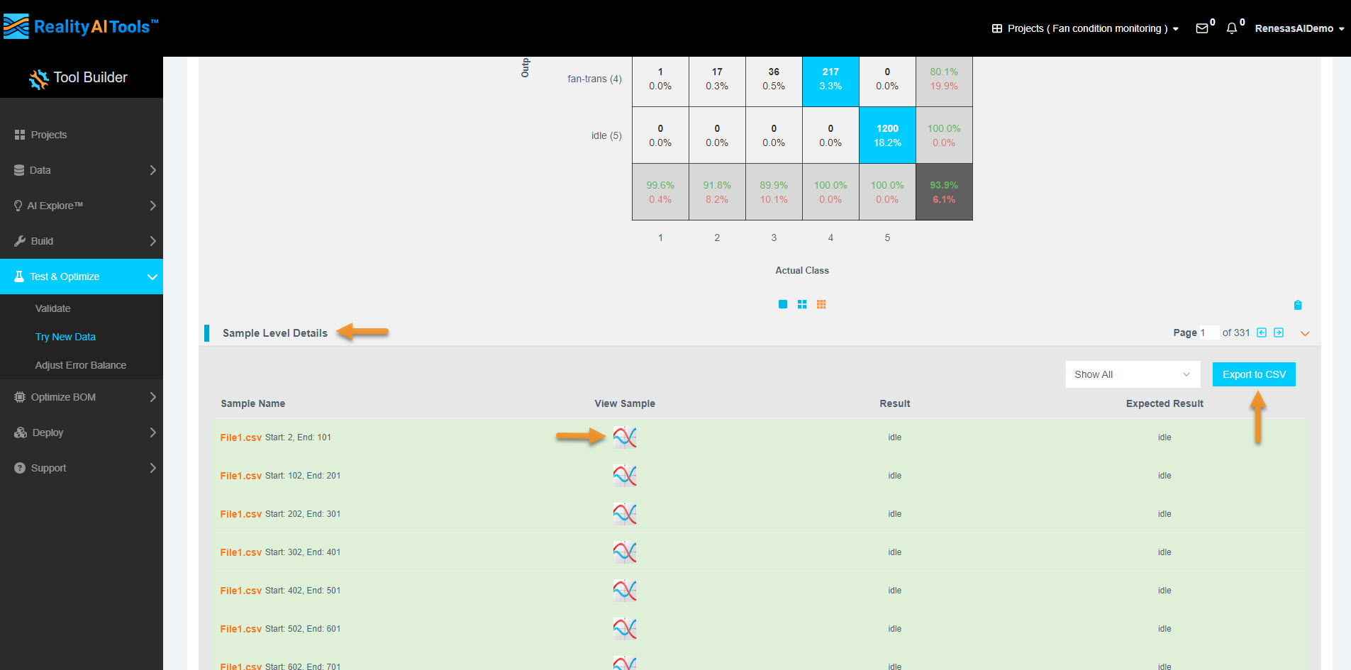
Terminology:
- Results: What the Reality AI Algorithm predicted.
- Expected Results: The labels assigned to the dataset (ground truth).
4.6 Viewing Waveforms (Optional)
- If you need to inspect the waveform of each data block/segment, go to the View Sample tab.
- This feature is useful for comparing the waveform of successful vs. unsuccessful predictions.
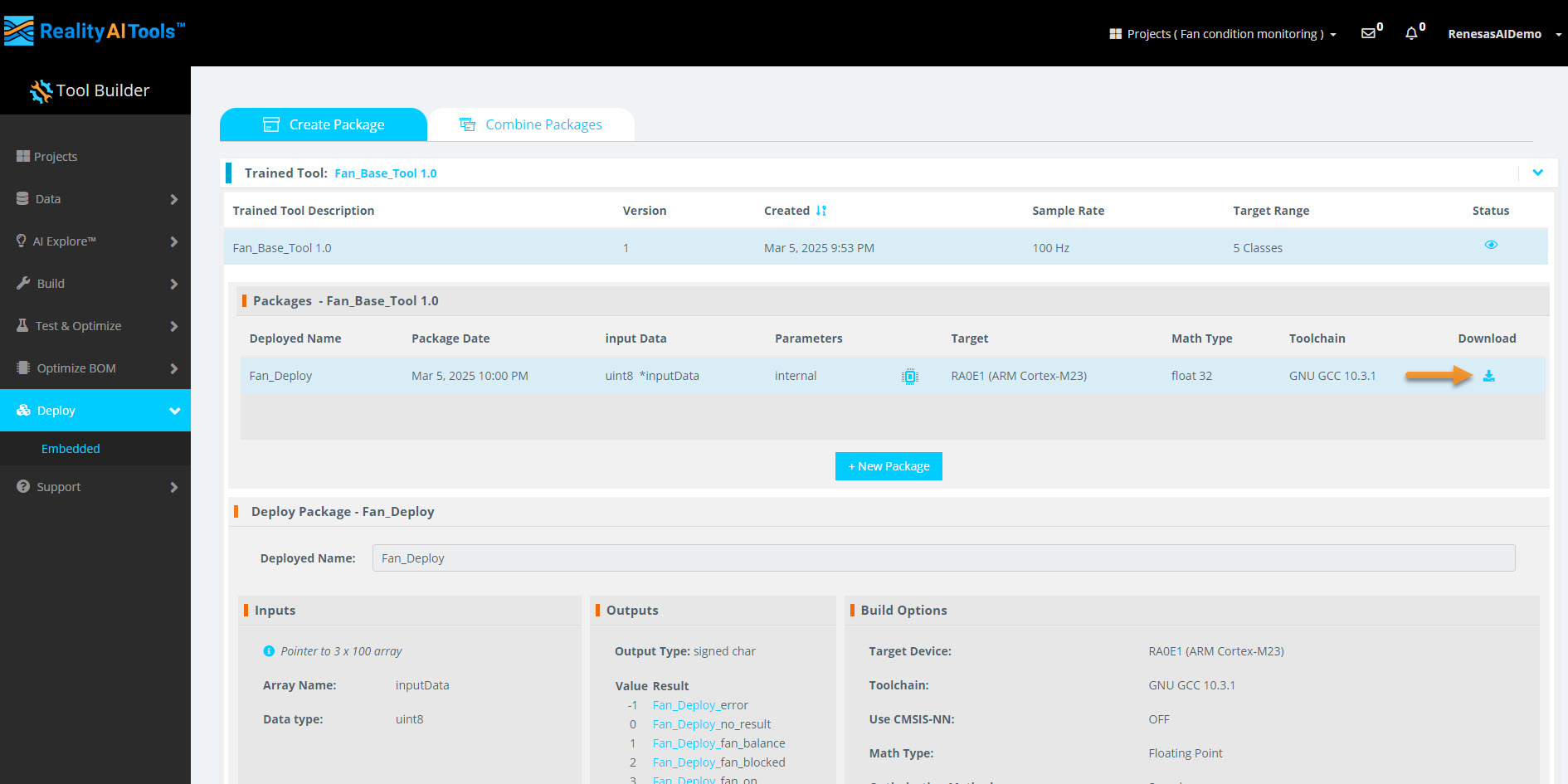
Step 5: Exporting the Model
In this section, we will export the trained model for deployment on a target embedded board.
5.1 Navigate to the Deployment Section
- In the left menu, go to Deploy & Embedded.
5.2 Create a New Package
- Select the model you previously exported (from Section 3).
- Click + New Package to start the export process.
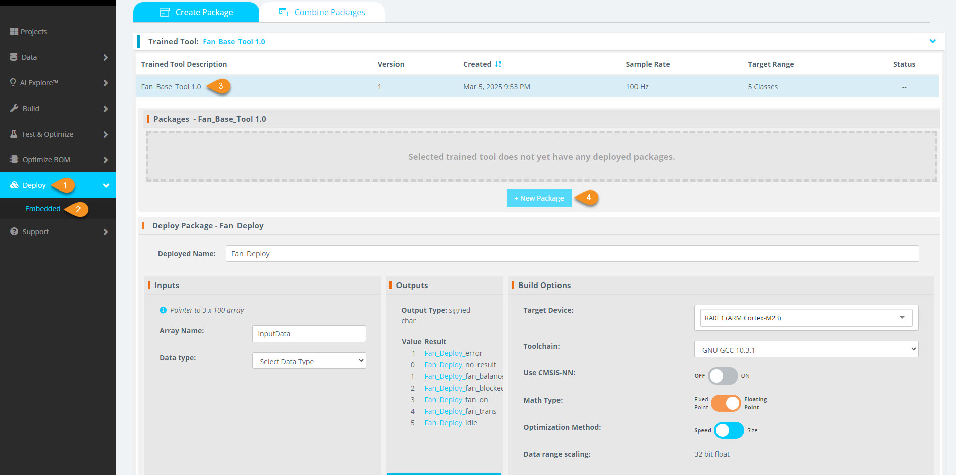
5.3 Configure the Export Package
- Name the exported package.
- Choose a Renesas processor from the available options.
5.4 Processor Variant Selection
- Select between FPU (Floating Point Unit) and non-FPU variants.
- Choose between soft and hard floating-point ABI.
5.5 Target Data Type Selection
- Select the target data type.
- For this tutorial, we will use int.
5.6 Generate the Deployment Package
-
Click Generate New Package to begin the export process.

-
The processing takes approximately 10-15 minutes.
-
Once completed, the buffering indicator will change to a download option.
-
Download the ZIP file containing the model deployment package.
5.7 Contents of the Downloaded ZIP File
The ZIP file contains multiple files necessary for deploying the model.
Key files include:
- examplemain.c – Function call of the model.
- size_report.txt – Provides resource consumption details for the selected processor.
5.8 Integrating the Model into Your Project
- Open examplemain.c to check the function call required for model execution.
- Integrate all the files into your IDE project to connect the model with your embedded system.
Model Execution in a Loop
- The model runs predictions on each window of data in a loop.
- It requires input data of the same window length as specified in Section 2.5 (e.g., 1 second or 100 data points).
5.9 Completion
You have successfully completed this section!