Using AI Live Monitor
To check the model accuracy:
-
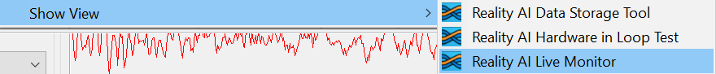
Navigate to Renesas AI > Reality AI > Show View > Reality AI Live Monitor.
Important: Disconnect the Data Storage Tool before proceeding.
-
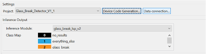
In the Settings section, the Project field displays the name of the currently selected project.
-
Click Device Code Generation... to open the Device Code Generation pop-up.
- After the model inference method and before the Data Shipper, insert the
RM_RAI_DATA_SHIPPER_Writemethod. - Copy the code using the Copy to Clipboard button in the pop-up and add it accordingly.
- After the model inference method and before the Data Shipper, insert the
-
Click Data Connection… to configure connection parameters.
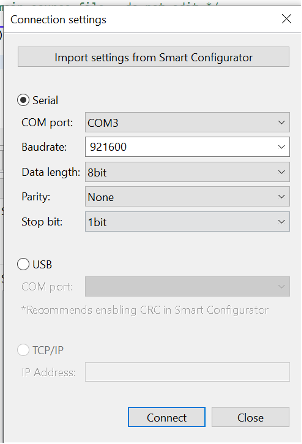
The Connection Settings pop-up appears.
-
Click Import setting from Smart Configurator.
This retrieves predefined connection parameters (instance ID, channel, name, format) from the Smart Configurator, minimizing manual input errors and ensuring compatibility with the hardware setup.
Setting Up the Connection
-
Select the appropriate connection type:
a. Serial Connection (Select Serial radio button)
- COM port: Choose the communication port assigned to the connected device.
- Baudrate: Defines data transmission speed; higher rates (e.g., 921600) allow faster transfer.
- Data Length: Number of bits in each packet (commonly 8 bits).
- Parity: Error checking option (None, Even, Odd).
- Stop Bit: Defines end of data packet; usually 1 stop bit, 2 for slower connections.
b. USB Connection (Select USB radio button)
- COM port: Select the required port.
- Recommendation: Enable CRC (Cyclic Redundancy Check) in the Smart Configurator for data integrity.
c. TCP/IP Connection (Select TCP/IP radio button)
- IP Address: Enter network IP address assigned to the device, allowing communication over a network.
-
Click Connect to start live model predictions.
-
In the Interference Output section, select the Interference Module from the dropdown.
The Class Map displays no results or specific classes based on the selected module. -
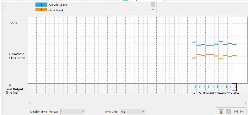
The Live Model Prediction Graph visualizes Normalized Class Scores (0–100%) on the Y-axis and Final Output Time (ms) on the X-axis.
Adjustable Parameters
Modify the graph display using these parameters:
- Display Time Interval: Select a time interval between 1 and 10 from the dropdown.
- Time Unit: Choose time unit from seconds (s), milliseconds (ms), microseconds (µs), or nanoseconds (ns).
- Chart Style: Select graph style: Stacked Chart, Bar Chart; for regression use cases, a Line chart is selected.
Graph Control Buttons
- Pause (||): Stops live graph updates.
- Play (>): Resumes live graph updates.
- Zoom Out (-): Decreases zoom level for broader view.
- Zoom In (+): Increases zoom for detailed view.
- Reset: Resets graph to default zoom and live update state.
Click Save to export data as a CSV file locally. You can also view the file in System Explorer.
- In the Result section, view:
- Total Monitored Time: Duration of model monitoring.
- Last Predictions Interval Time: Duration of most recent prediction interval.
- Average Predictions Interval Time: Average time between predictions.